
Ph.D. in Computer Engineering, Data Scientist
Precision and Recall
LearnDataSci is reader-supported. When you purchase through links on our site, earned commissions help support our team of writers, researchers, and designers at no extra cost to you.
What is Precision and Recall?
Precision and Recall are metrics used to evaluate machine learning algorithms since accuracy alone is not sufficient to understand the performance of classification models.
Suppose we developed a classification model to diagnose a rare disease, such as cancer. If only 5% of patients have cancer, a model that predicts all patients are healthy will have 95% accuracy. If only 0.1% of patients have cancer, the same model predicting all patients are healthy achieves 99.9% accuracy. Of course, the "accuracy" is misleading. Both these models are useless for detecting disease because they miss all cancers! We need other metrics that help us weigh the cost of different types of errors.
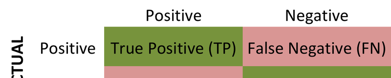
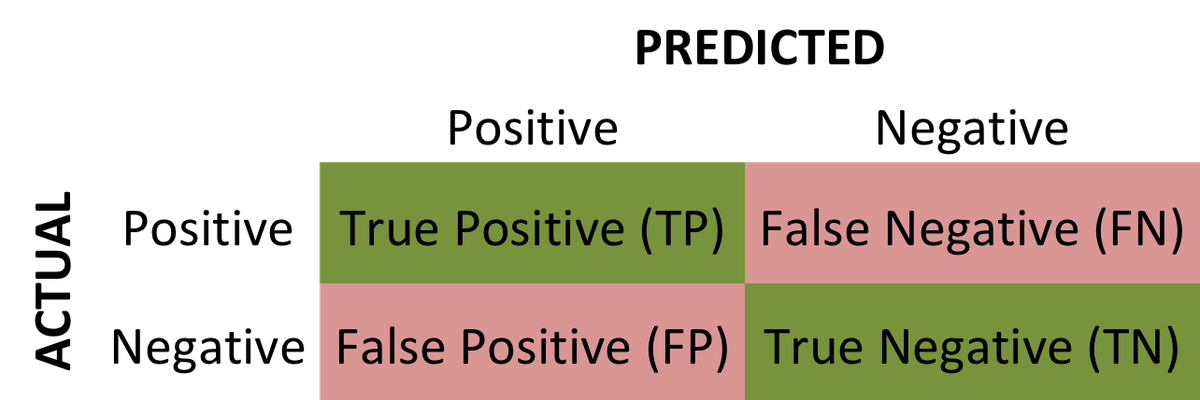
We can create a confusion matrix to represent the results of a binary classification.
How to Calculate Precision, Recall, and F1 Score
Precision gives the proportion of positive predictions that are actually correct. It takes into account false positives, which are cases that were incorrectly flagged for inclusion. Precision can be calculated as:
$$ Precision = \frac{TP}{TP + FP}$$
Recall measures the proportion of actual positives that were predicted correctly. It takes into account false negatives, which are cases that should have been flagged for inclusion but weren't. Recall can be calculated as:
$$ Recall = \frac{TP}{TP + FN}$$
Consider a system designed to distinguish real email from spam. In this system, a real email message is a true positive. A model that throws away all emails as spam will have perfect precision because there are no false positives (no emails incorrectly flagged as real). However, Recall will be 0% because there are no true positives (no emails correctly flagged as real).
A good model needs to strike the right balance between Precision and Recall. For this reason, an F-score (F-measure or F1) is used by combining Precision and Recall to obtain a balanced classification model. F-score is calculated by the harmonic mean of Precision and Recall as in the following equation.
$$ F-score = 2 \times \frac{p \times r}{ p + r} $$
We can also use Precision and Recall for multi-class problems. A confusion matrix can be constructed to represent the results of a 3-class model.
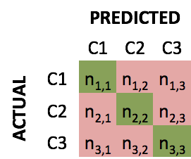
We can calculate the Accuracy of the model as follows:
$ \textrm{Accuracy of the model} = \frac{\textrm{What the model predicted correctly}}{\textrm{Total number of elements}} = \frac {n_{1,1} +n_{2,2} + n_{2,2} }{N} $
Precison and Recall for each class are calculated separately. For example, Precision and Recall for Class 1 is computed as follows:
$ \textrm{Precision of the model for C1} = \frac{\textrm{What the model predicted correctly as C1}}{\textrm{What the model predicted as C1}} = \frac {n_{1,1} }{n_{1,1}+n_{2,1} + n_{3,1}} $
$ \textrm{Recall of the model for C1} = \frac{\textrm{What the model predicted correctly as C1}}{\textrm{What is actually C1}} = \frac {n_{1,1} }{n_{1,1}+n_{1,2} + n_{1,3}} $
Precision and Recall are calculated for Class 2 and Class 3 in the same way. For data with more than 3 classes, the metrics are calculated using the same methodology.
A Python Example
Let's use a sample data set to show the calculation of evaluation metrics. Our goal is to predict whether the tumor is malignant from the size of the tumor in the breast cancer data.
This dataset has two classes: malignant, denoted as 0, and benign, denoted as 1. Because the target is a binary variable, this is a binary classification problem. This example will use a simple method for binary classification.
If the mean area of tumor is higher than a defined threshold, the model will classify the objects as malignant. We will create a function from scratch to calculate the evaluation metrics.
First, we will import and load the dataset:
import numpy as np
from sklearn.datasets import load_breast_cancer
dataset = load_breast_cancer()Next, we define the predictor and target variables:
x = dataset['data'][:,3] # Column 3 is mean area of the tumor
y = dataset['target']
# Apply min-max normalization
x = (x - np.min(x)) / (np.max(x) - np.min(x) )Now, we can define a simple classifier:
def a_simple_classifier(x, thres = 0.5):
predicted = np.zeros(len(x))
for i in range(len(x)):
if x[i] < thres:
predicted[i] = 1
return predictedHere, we'll create the function to obtain the values for Accuracy, Precision, Recall, and F1 Score:
def calculate_metrics(predicted, actual):
TP, FP, TN, FN = 0, 0, 0, 0
for i in range(len(predicted)):
if (predicted[i] == 0) & (actual[i] == 0):
TP += 1
elif (predicted[i] == 0) & (actual[i] == 1):
FP += 1
elif (predicted[i] == 1) & (actual[i] == 1):
TN += 1
else:
FN += 1
accuracy = (TP + TN) / (TP + FP + TN + FN)
precision = (TP) / (TP + FP)
recall = (TP) / (TP + FN)
f1_score = (2 * precision * recall) / (precision + recall)
return accuracy, precision, recall, f1_scoreWe'll now apply the classifier defined above for different threshold values. We defined 20 different threshold values using np.linspace and an array for each metric. Then, we loop through each threshold value, get a prediction from our classifier, get each metric, and print a column for each result.
thresh = np.linspace(0,1,20)
accuracy = np.zeros(len(thresh))
precision = np.zeros(len(thresh))
recall = np.zeros(len(thresh))
f1_score = np.zeros(len(thresh))
print('Threshold \t Accuracy \t Precision\t Recall \t F1 Score ')
for i in range(len(thresh)):
prediction = a_simple_classifier(x, thresh[i])
accuracy[i], precision[i], recall[i], f1_score[i]=calculate_metrics(prediction, y)
print(f'{thresh[i]: .2f}\t\t {accuracy[i]: .2f}\t\t {precision[i]: .2f}\t\t {recall[i]: .2f}\t\t {f1_score[i]: .2f}')Threshold Accuracy Precision Recall F1 Score
0.00 0.37 0.37 1.00 0.54
0.05 0.41 0.39 1.00 0.56
0.11 0.55 0.45 0.99 0.62
0.16 0.78 0.63 0.94 0.76
0.21 0.86 0.81 0.83 0.82
0.26 0.86 0.96 0.67 0.79
0.32 0.83 0.99 0.56 0.71
0.37 0.78 1.00 0.42 0.59
0.42 0.75 1.00 0.32 0.49
0.47 0.70 1.00 0.19 0.32
0.53 0.66 1.00 0.10 0.18
0.58 0.65 1.00 0.07 0.12
0.63 0.65 1.00 0.06 0.11
0.68 0.64 1.00 0.03 0.06
0.74 0.63 1.00 0.02 0.04
0.79 0.63 1.00 0.02 0.04
0.84 0.63 1.00 0.01 0.03
0.89 0.63 1.00 0.01 0.02
0.95 0.63 1.00 0.01 0.02
1.00 0.63 1.00 0.00 0.01Results show the effect of changing the threshold. Increasing the threshold enhances Precision and decreases Recall. The F1 Score balancing precision with Recall was highest at a threshold of .21.
The following graph plots Precision versus Recall to see the changes with respect to each other.
import matplotlib.pyplot as plt
plt.plot(precision, recall)
plt.xlabel('Precision')
plt.ylabel('Recall')
plt.title('Precision versus Recall')
plt.show()
The figure shows that the Precision and Recall values are inversely related. As one increases, the other decreases.
We'll also plot a graph to show the changes of all metrics togther:
plt.plot(thresh, accuracy, 'r')
plt.plot(thresh, precision, 'g')
plt.plot(thresh, recall,'b')
plt.plot(thresh, f1_score,'k')
plt.legend(['Accuracy', 'Precision','Recall', 'F1 Score' ])
plt.xlabel('Threshold')
plt.ylabel('Scores')
plt.title('Change of Evaluation Metrics according to Threshold')
plt.show()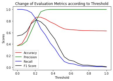
The most meaningful value to consider in the above graph is the F1 score (black line). The highest value of F1 score is where the Precision and Recall values are close to each other. F1 score is optimum when the threshold value is 0.21.
Multi-Class Model Evaluation
In this example, we'll use the Iris dataset to create a multi-class model for classifying different species of iris flowers. This dataset consists of 3 different types of Iris flowers (Setosa, Versicolour, and Virginica). The features are Sepal Length, Sepal Width, Petal Length, and Petal Width.
For this example, we will use the Scikit-Learn library to evaluate the classification model.
First, we'll import and load the dataset:
from sklearn.datasets import load_iris
dataset = load_iris()We'll now go through five steps to create the model and obtain the required metrics.
Step 1: Define explanatory variables and target variable.
X = dataset['data']
y = dataset['target']Step 2: Apply normalization operation for numerical stability.
from sklearn.preprocessing import StandardScaler
standardizer = StandardScaler()
X = standardizer.fit_transform(X)Step 3: Fit Logistic Regression Model to the train data.
from sklearn.linear_model import LogisticRegression
model = LogisticRegression()Step 4: Make predictions on the data using cross-validation.
from sklearn.model_selection import cross_val_predict
y_pred = cross_val_predict(model, X, y, cv=10)Step 5: Calculate the Confusion Matrix by the actual and predicted values.
from sklearn.metrics import confusion_matrix
conf_mat = confusion_matrix(y, y_pred)Finally, we can create a heatmap to show the confusion matrix:
import seaborn as sns
sns.heatmap(conf_mat, annot=True)
plt.xlabel("Predicted Label")
plt.ylabel('Actual Label')
plt.title('Confusion matrix of the model')
plt.show()Additionally, let's print the classification report to observe the evaluation metrics:
from sklearn.metrics import classification_report
print(classification_report(y, y_pred))precision recall f1-score support
0 0.99 0.96 0.97 212
1 0.98 0.99 0.98 357
accuracy 0.98 569
macro avg 0.98 0.98 0.98 569
weighted avg 0.98 0.98 0.98 569From the classification report, we can observe the values of the evaluation metrics for each class and the average of each metric. For example, the precision and recall of the model for Class 0 are both 1.00, which means that the model can accurately predict all instances of Class 0.
Note that the report gives the number of instances for each class. macro avg and weighted avg are the unweighted mean and weighted mean relative to support, respectively.
Furthermore, the sklearn library has separate functions for each evaluation metric, which you can find in their docs here.
Below are examples of how to calculate each metric individually using sklearn:
from sklearn.metrics import precision_score, recall_score, f1_score, accuracy_score
print('Accuracy: ', accuracy_score(y, y_pred))
print('Precision:', precision_score(y, y_pred, average='macro'))
print('Recall: ', recall_score(y, y_pred, average='macro'))
print('F1 Score: ', f1_score(y, y_pred, average='macro'))Accuracy: 0.9806678383128296
Precision: 0.9817038994314997
Recall: 0.9769303947994292
F1 Score: 0.9792239951404265The above evaluation metrics give the averages of the classes. If we want to observe the precision for each class separately, we need to define the labels parameter. An example for Class 1 is given below.
print('Precision for Class 1:', precision_score(y, y_pred, average='macro', labels=[1]))
print('Recall for Class 1 :', recall_score(y, y_pred, average='macro', labels=[1]))Precision for Class 1: 0.9779005524861878
Recall for Class 1 : 0.9915966386554622Meet the Authors

Associate Professor of Computer Engineering. Author/co-author of over 30 journal publications. Instructor of graduate/undergraduate courses. Supervisor of Graduate thesis. Consultant to IT Companies.

