

Ph.D. in Computer Engineering, Data Scientist
Orthogonal and Orthonormal Vectors
LearnDataSci is reader-supported. When you purchase through links on our site, earned commissions help support our team of writers, researchers, and designers at no extra cost to you.
You should already know:
- Basic vector and matrix math. Learn these concepts in Brilliant's Linear Algebra series.
What are orthogonal vectors?
Two vectors $u$ and $v$ are considered to be orthogonal when the angle between them is $90^\circ$. In other words, orthogonal vectors are perpendicular to each other. Orthogonality is denoted by $ u \perp v$.
A set of vectors $S=\{v_1,v_2, v_3...v_n\}$ is mutually orthogonal if every vector in the set $S$ is perpendicular to each other.
That is, sets are mutually orthogonal when each combination/pair of vectors within the set are orthogonal to each other. i.e., $ v_i \perp v_j$.
Another characteristic of orthogonal vectors is that their dot product ($u \cdot v$) equals zero. The dot product of two vectors $u = [u_1, u_2, ...u_n]$ and $v=[v_1, v_2... v_n]$ is calculated as follows: $$ \large \begin{align} u \cdot v &= u^T v \\[2pt] &= \sum_{i=1} ^{n} u_iv_i \\[2pt] &= u_1v_1 + u_2v_2 + ...+ u_nv_n \\[2pt] &= \|u\|\|v\| \cos \theta \\[2pt] \end{align} $$
In the above equation:
- $u^T$ represents the transpose of the vector $u$.
- $\|u\|$ represent the L2 norm (magnitude) of the vector, meaning the root of the squared elements. $\|u\| = \sqrt{u_1^2 + u_2^2 ... u_n^2}$
- $\theta$ is the angle between the vectors.
To see why the dot product between two vectors is $0$ when they are orthogonal (perpendicular), recall that $\cos 90^\circ = 0$, which causes the dot product in the previous equation to be $0$:
$$ u \cdot v = \|u\|\|v\|\cos 90^\circ = \|u\|\|v\|(0) = 0 $$
Orthogonal matrices
An orthogonal matrix is a square matrix (the same number of rows as columns) whose rows and columns are orthogonal to each other. A special property of any orthogonal matrix is that its transpose is equal to its inverse. Another notable property is that the product of any orthogonal matrix and its transpose gives the identity matrix $I$. Last but not least, the transpose of an orthogonal matrix is also always orthogonal.
$$ A^T A = A A^T = I $$ $$ A^T = A^{-1} $$

What are orthonormal vectors?
Orthonormal vectors are a special instance of orthogonal vectors. In addition to having a $90^\circ$ angle between them, orthonormal vectors each have a magnitude of 1. In particular, the following three conditions must be met:
- $ u \cdot v =0$
- $\|u\| =1$
- $\|v\| =1 $
In Data Science and Machine Learning, orthogonal vectors and matrices are often used to develop more advanced methods. They have many convenient characteristics that make them a helpful tool. For example, the inverse of an orthogonal matrix is easy to calculate. Some methods employing orthogonal vectors or matrices include:
- Singular Value Decomposition (SVD). SVD is a popular method used for dimensionality reduction
- Regularization of a convolution layer to train Deep Neural Networks. These methods are called Orthogonal Deep Neural Networks and Orthogonal Convolutional Neural Networks.
- Haar Transform. A method used for compressing digital images.
Example 1:
Consider the following two vectors in 2D space: $$ v_1 = \begin{bmatrix} 1 \\ 2 \end{bmatrix}, \space v_2 = \begin{bmatrix} 2 \\ -1\end{bmatrix}$$ The dot product of these vectors is: $$ v_1 \cdot v_2 = v_1^T v_2 = (1\times 2) +(2 \times -1) = 0$$ Because the dot product is zero, the angle between the vectors is $90^\circ$ ($ \cos 90 ^{\circ} = 0$ ). Therefore, these two vectors are orthogonal.
Example 2:
Consider the following three vectors in 3D space: $$ v_1 = \begin{bmatrix} 2 \\ 0 \\ 2 \end{bmatrix}, \space v_2 = \begin{bmatrix} -3 \\ 0 \\ 3 \end{bmatrix}, \space v_3 = \begin{bmatrix} 0 \\ 5 \\ 0 \end{bmatrix} \space $$ The dot product of these vectors is: $$ v_1 \cdot v_2 = v_1^T v_2 = (2\times -3) + (0 \times 0) + (2 \times 3) = 0 $$ $$ v_1 \cdot v_3 = v_1^T v_3 = (2\times 0) + (0 \times 5) + (2 \times 0) = 0 $$ $$ v_2 \cdot v_3 = v_2^T v_3 = (-3\times 0) + (0 \times 5) + (3 \times 0) = 0 $$
Because the dot products are all zero, these three vectors are mutually orthogonal.
Example 3:
The $N \times N$ Haar transformation matrix for $N=2$ and $N=4$ can be defined as follows.
$$ H_2 = \frac{1}{\sqrt2} \begin{bmatrix} 1& 1 \\ 1 & -1 \end{bmatrix} $$
$$ H_4 = \frac{1}{\sqrt4} \begin{bmatrix} 1& 1& 1 &1 \\ 1 &1& -1& -1 \\ \sqrt 2 & -\sqrt 2& 0& 0 \\ 0&0&\sqrt 2 &-\sqrt2 \end{bmatrix} $$
The transpose of the matrix is equal to its inverse ($H^{-1} = H^T$ and $HH^T =I$). Because all columns and rows are orthogonal to each other, and because the magnitude of all rows and columns are equal to one, this matrix is also orthonormal.
Python Example 1
In Python programming, the numpy library has useful linear algebra functions such as transpose, dot product, magnitude, and norm (see our NumPy Tutorial). Some examples are given below to show the orthogonality of a vector.
import numpy as np
import matplotlib.pyplot as plt
from mpl_toolkits.mplot3d import Axes3DFirst, we'll create two vectors:
v1 = np.array([1,-2, 4])
v2 = np.array([2, 5, 2])We can perform the dot product of the vectors using standard calculation:
dot_product = np.sum(v1 * v2)
print("The dot product of v1 and v2 is", dot_product )The dot product of v1 and v2 is 0Since the dot product is 0, the vectors are orthogonal.
Numpy also contains a dot product function, which we can use like so:
dot_product = np.dot(v1,v2)
print("The dot product of v1 and v2 is", dot_product )The dot product of v1 and v2 is 0Let's also calculate the length of each vector using the formula given above:
n1 = np.sqrt(np.sum(v1 * v1))
n2 = np.sqrt(np.sum(v2 * v2))
print('The L2 norm of v1 is', n1)
print('The L2 norm of v2 is', n2)The L2 norm of v1 is 4.58257569495584
The L2 norm of v2 is 5.744562646538029Alternatively, the length of a vector can be calculated using the L2 norm function builtin to Numpy:
n1 = np.linalg.norm(v1, ord=2)
n2 = np.linalg.norm(v2, ord=2)
print('The L2 norm of v1 is', n1)
print('The L2 norm of v2 is', n2)The L2 norm of v1 is 4.58257569495584
The L2 norm of v2 is 5.744562646538029The dot product of the two vectors is 0, but the L2 norm of each vector is not equal to 1. This tells us that these vectors are orthogonal but not orthonormal.
Python Example 2
We will now define the Haar transform matrix:
haar_matrix = (1/2) * np.array([[1, 1, 1, 1],
[1, 1, -1, -1],
[np.sqrt(2), -np.sqrt(2), 0,0],
[0, 0, np.sqrt(2), -np.sqrt(2)]]
)
print("4D Haar Transform Matrix is : \n", haar_matrix)4D Haar Transform Matrix is :
[[ 0.5 0.5 0.5 0.5 ]
[ 0.5 0.5 -0.5 -0.5 ]
[ 0.70710678 -0.70710678 0. 0. ]
[ 0. 0. 0.70710678 -0.70710678]]And then calculate the dot product:
dot_haar = np.dot(haar_matrix,np.transpose(haar_matrix))
print("The Dot Product of the 4D Haar Matrix is:\n", dot_haar)The Dot Product of the 4D Haar Matrix is:
[[1. 0. 0. 0.]
[0. 1. 0. 0.]
[0. 0. 1. 0.]
[0. 0. 0. 1.]]The dot product of the Haar transform matrix and its transpose gives the identity matrix. Because all rows and columns are orthogonal, the results of the dot products (non-diagnoal elements of the matrix) are all zeros. Because the diagonal elements of the matrix are equal to one, this matrix is also orthonormal.
Visualization of Orthogonal Vectors
First, a 2D representation of orthogonal vectors.
fig = plt.figure(figsize=(5, 5))
ax = fig.add_subplot(111)
ax.grid(alpha=0.4)
ax.set(xlim=(-3, 3), ylim=(-3, 3))
v1 = np.array([1, 2])
v2 = np.array([2, -1])
# Plot the orthogonal vectors
ax.annotate('', xy=v1, xytext=(0, 0), arrowprops=dict(facecolor='r'))
ax.annotate('', xy=v2, xytext=(0, 0), arrowprops=dict(facecolor='g'))
plt.show()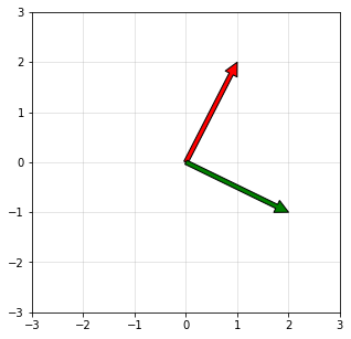
And here's an example of orthogonal vectors in 3D space.
# 3D representation of the orthogonal vectors
fig = plt.figure(figsize=(8, 8))
ax = fig.add_subplot(111, projection='3d')
# Define the orthogonal vectors
v1 = np.array([ 0, 0, -1])
v2 = np.array([ 1, 1, 0])
v3 = np.array([-1, 1, 0])
# Plot the orthogonal vectors
ax.quiver( 0, 0, 0, v1[0], v1[1], v1[2], color = 'r', lw=3, arrow_length_ratio=0.2)
ax.quiver( 0, 0, 0, v2[0], v2[1], v2[2], color = 'g', lw=3, arrow_length_ratio=0.2)
ax.quiver( 0, 0, 0, v3[0], v3[1], v3[2], color = 'b', lw=3, arrow_length_ratio=0.2)
ax.set_xlim([-1, 1]), ax.set_ylim([-1, 1]), ax.set_zlim([-1, 1])
ax.set_xlabel('X axis'), ax.set_ylabel('Y axis'), ax.set_zlabel('Z axis')
plt.show()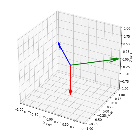
Meet the Authors

Associate Professor of Computer Engineering. Author/co-author of over 30 journal publications. Instructor of graduate/undergraduate courses. Supervisor of Graduate thesis. Consultant to IT Companies.