
Data Science Consultant
Convolutional Neural Networks — Image Classification w. Keras
LearnDataSci is reader-supported. When you purchase through links on our site, earned commissions help support our team of writers, researchers, and designers at no extra cost to you.
You should already know:
You should be fairly comfortable with Python and have a basic grasp of regular Neural Networks for this tutorial. The Neural Networks and Deep Learning course on Coursera is a great place to start.
Introduction to Image Classification
There's no shortage of smartphone apps today that perform some sort of Computer Vision task. Computer Vision is a domain of Deep Learning that centers on the fundamental problem in training a computer to see as a human does.
The way in which we perceive the world is not an easy feat to replicate in just a few lines of code. We are constantly recognizing, segmenting, and inferring objects and faces that pass our vision. Subconsciously taking in information, the human eye is a marvel in itself. Computer Vision deals in studying the phenomenon of human vision and perception by tackling several 'tasks', to name just a few:
- Object Detection
- Image Classification
- Image Reconstruction
- Face Recognition
- Semantic Segmentation
The research behind these tasks is growing at an exponential rate, given our digital age. The accessibility of high-resolution imagery through smartphones is unprecedented, and what better way to leverage this surplus of data than by studying it in the context of Deep Learning.
In this article, we will tackle one of the Computer Vision tasks mentioned above, Image Classification.
Image Classification attempts to connect an image to a set of class labels. It is a supervised learning problem, wherein a set of pre-labeled training data is fed to a machine learning algorithm. This algorithm attempts| to learn the visual features contained in the training images associated with each label, and classify unlabelled images accordingly. It is a very popular task that we will be exploring today using the Keras Open-Source Library for Deep Learning.
The first half of this article is dedicated to understanding how Convolutional Neural Networks are constructed, and the second half dives into the creation of a CNN in Keras to predict different kinds of food images. Click here to skip to Keras implementation.
Let's get started!
Neural Network Architecture
This article aims to introduce convolutional neural networks, so we'll provide a quick review of some key concepts.
Neural Network Layers:
Neural networks are composed of 3 types of layers: a single Input layer, Hidden layers, and a single output layer. Input layers are made of nodes, which take the input vector's values and feeds them into the dense, hidden-layers.
The number of hidden layers could be quite large, depending on the nature of the data and the classification problem. The hidden layers are fully-connected in that a single node in one layer is connected to all nodes in the next layer via a series of channels.
Input values are transmitted forward until they reach the Output layer. The Output layer is composed of nodes associated with the classes the network is predicting.
Forward Propagation:
When data is passed into a network, it is propagated forward via a series of channels that are connecting our Input, Hidden, and Output layers. The values of the input data are transformed within these hidden layers of neurons.
Recall that each neuron in the network receives its input from all neurons in the previous layer via connected channels. This input is a weighted sum of all the weights at each of these connections, multiplied by the previous layer's output vector. This weighted sum is passed to an Activation Function, which results in the output for a particular neuron and the input for the next layer. This forward propagation happens for each layer until data reaches the Output layer - where the number of neurons corresponds to the number of classes that are being predicted.
Backpropagation:
Once the Output layer is reached, the neuron with the highest activation would be the model's predicted class. Loss is calculated given the output of the network and results in a magnitude of change that needs to occur in the output layer to minimize the loss.
Neural networks attempt to increase the value of the output node according to the correct class. This is done through backpropagation. In backpropagation, the derivative (i.e. gradients) of the loss function with respect to each hidden layer's weights are used to increase the value of the correct output node. Gradient descent seeks to minimize the overall loss that is being calculated for the network's predictions.
This has been a high-level explanation of regular neural networks. It does not cover the different types of Activation or Loss functions that are used in applications. Before proceeding through this article, it's recommended that these concepts are comprehensively understood.
How Does a Computer See?
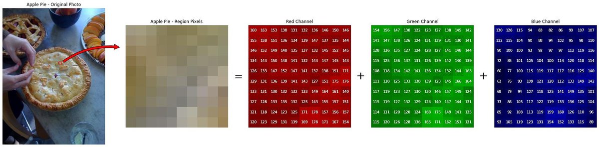
Before we dive into image classification, we need to understand how images are represented as data. Consider this image of a fruit bowl. As humans, we can clearly distinguish a banana from an orange. The visual features that we use (color, shape, size) are not represented the same way when fed to an algorithm.
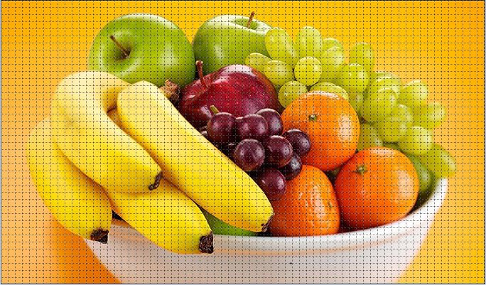
Digital images are composed of a grid of pixels. An image's pixels are valued between 0 and 255 to represent the intensity of light present. Therefore, we can think of the fruit bowl image above as a matrix of numerical values. This matrix has two axes, X and Y (i.e. the width and height.
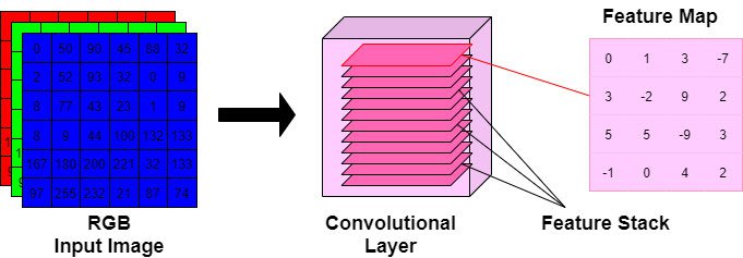
Color images are constructed according to the RGB model and have a third dimension - depth. Color images are a 3-Dimensional matrix of red, green, and blue light-intensity values. These color channels are stacked along the Z-axis.
The dimensions of this fruit bowl image are 400 x 682 x 3. The width and height are 682 and 400 pixels, respectively. The depth is 3, as this is an RGB image.
In this article, we're going to learn how to use this representation of an image as an input to a deep learning algorithm, so it's important to remember that each image is constructed out of matrices.
Behind the scenes, the edges and colors visible to the human eye are actually numerical values associated with each pixel. A high-resolution image will have a high number of pixels, and therefore a larger set of matrices.
Convolutional Neural Networks
Recall the functionalities of regular neural networks. Input data is represented as a single vector, and the values are forward propagated through a series of fully-connected hidden layers. The Input layer of a neural network is made of $N$ nodes, where $N$ is the input vector's length. Further computations are performed and transform the inputted data to make a prediction in the Output layer. The number of features is an important factor in how our network is designed.
Suppose we have a 32-pixel image with dimensions [32x32x3]. Flattening this matrix into a single input vector would result in an array of $32 \times 32 \times 3=3,072$ nodes and associated weights.
This could be a manageable input for a regular network, but our fruit bowl image may not be so manageable! Flattening its dimensions would result in $682 \times 400 \times 3=818,400$ values. Time and computation power simply do not favor this approach for image classification.
Convolutional Neural Networks (CNNs) have emerged as a solution to this problem. You'll find this subclass of deep neural networks powering almost every computer vision application out there! High-resolution photography is accessible to almost anyone with a smartphone these days.
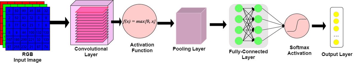
Architecture
CNN architectures are made up of some distinct layers. In all cases, the layers take as input a 3D volume, transform this volume through differential equations, and output a 3D volume. Some layers require the tweaking of hyperparameters, and some do not.
0. Input Layer:
- the raw pixel values of an image represented as a 3D matrix
- Dimensions $W$ x $H$ x $D$, where depth corresponds to the number of color channels in the image.
1. Convolutional Layer:
- Conv. Layers will compute the output of nodes that are connected to local regions of the input matrix.
- Dot products are calculated between a set of weights (commonly called a filter) and the values associated with a local region of the input.
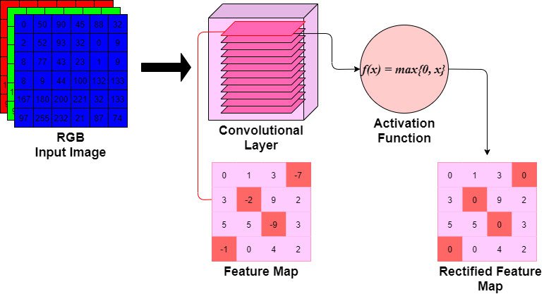
2. ReLu (Activation) Layer:
- The output volume of the Conv. layer is fed to an elementwise activation function, commonly a Rectified-Linear Unit (ReLu).
- The ReLu layer will determine whether an input node will 'fire' given the input data.
- This 'firing' signals whether the convolution layer's filters have detected a visual feature.
- A ReLu function will apply a $max(0,x)$ function, thresholding at 0.
- The dimensions of the volume are left unchanged.
3. Pooling Layer:
- A down-sampling strategy is applied to reduce the width and height of the output volume.
4. Fully-Connected Layer:
- The output volume, i.e. 'convolved features,' are passed to a Fully-Connected Layer of nodes.
- Like conventional neural-networks, every node in this layer is connected to every node in the volume of features being fed-forward.
- The class probabilities are computed and are outputted in a 3D array with dimensions: [$1$x$1$x$K$], where $K$ is the number of classes.
Let's go through each of these one-by-one.
1. Convolutional Layers
Let's say you're looking at a photograph, but instead of seeing the photograph as a whole, you start by inspecting the photograph from the top left corner and begin moving to the right until you've reached the end of the photograph. You move down the line, and begin scanning left to right again. Every time you shift to a new portion of the photo, you take in new information about the image's contents. This is sort of how convolution works.
Convolutional layers are the building blocks of CNNs. These layers are made of many filters, which are defined by their width, height, and depth. Unlike the dense layers of regular neural networks, Convolutional layers are constructed out of neurons in 3-Dimensions. Because of this characteristic, Convolutional Neural Networks are a sensible solution for image classification.
1.1 Filters
Convolutional Layers are composed of weighted matrices called Filters, sometimes referred to as kernels.
Filters slide across the image from left-to-right, taking as input only a subarea of the image (the receptive field). We will see how this local connectivity between activated nodes and weights will optimize neural network's performance as a whole.
Filters have a width and height. Many powerful CNN's will have filters that range in size: 3 x 3, 5 x 5, in some cases 11 x 11. These dimensions determine the size of the receptive field of vision.
The depth of a filter is equal to the number of filters in the convolutional layer.
Filters will activate when the elementwise multiplication results in high, positive values. This informs the network of the presence of something in the image, such as an edge or blotch of color.
The values of the outputted feature map can be calculated with the following convolution formula:
$$G[m,n] = (f * h)[m,n] = \sum_j\sum_kh[j, k]f[m - j, n - k]$$ where the input image is denoted by f, the filter by h, and the m and n represent the indexes of rows and columns of the outputted matrix. The $*$ operator is a special kind of matrix multiplication.
If you're interested in see an example convolution done out by hand, see this.
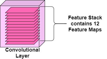
This computation occurs for every filter within a layer. The outputted feature maps can be thought of as a feature stack.
Filter hyperparameters
Filters have hyperparameters that will impact the size of the output volume for each filter.
1. Stride: the distance the filter moves at a time. A filter with a stride of 1 will move over the input image, 1 pixel at a time.
2. Padding: a zero-padding scheme will 'pad' the edges of the output volume with zeros to preserve spatial information of the image (more on this below).
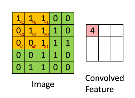
Consider Figure 5., with an input image size of 5 x 5 and a filter size of 3 x 3. We can calculate the size of the resulting image with the following formula:
$$(n - f + 1) * (n - f + 1)$$
Where $n$ is the input image size and $f$ is the size of the filter. We can plug in the values from Figure 5 and see the resulting image is of size 3:
$$(n - f + 1) = (5-3) + 1 = 3$$
The size of the resulting feature map would have smaller dimensions than the original input image. This could be detrimental to the model's predictions, as our features will continue to pass through many more convolutional layers. How do we ensure that we do not miss out on any vital information?
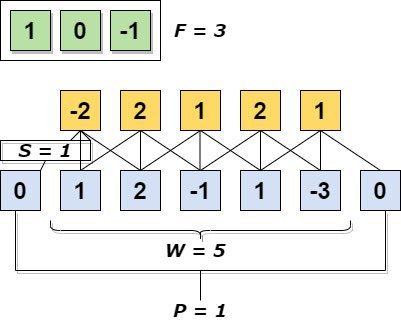
When we incorporate stride and padding into the process, we ensure that our input and output volumes remain the same size - thus maintaining the spatial arrangement of visual features. Output volume size can be calculated as a function of the Input volume size:
$$\frac{W - F + 2P}{S + 1}$$
Where:
- $W$ is the size of the Input volume,
- $F$ the receptive field size of the Convolutional layer filters,
- $P$ is the amount of zero-padding used about the border of the output matrix,
- and $S$ is the stride of the filter.
In the graphical representation below, the true input size ($W$) is 5. Our zero-padding scheme is $P = 1$, the stride $S = 1$, and the receptive field of $F = 3$ contains the weights we will use to obtain our dot products. We can see how zero-padding around the edges of the input matrix helps preserve the original input shape. If we were to remove zero-padding, our output would be size 3. As convolution continues, the output volume would eventually be reduced to the point that spatial contexts of features are erased entirely. This is why zero-padding is important in convolution.
1.2 Parameter Sharing
Recall the image of the fruit bowl. Say we resize the image to have a shape of 224x224x3, and we have a convolutional layer, where the filter size is a 5 x 5 window, a stride = 2, and padding = 1. In this convolutional layer, the depth (i.e. the number of filters) is set to 64.
Now given our fruit bowl image, we can compute $\frac{(224 - 5)}{2 + 1} = 73$.
Since the convolutional layer's depth is 64, the Convolutional output volume will have a size of [73x73x64] - totalling at 341,056 neurons in the first convolutional layer.
Each of the 341,056 neurons is connected to a region of size [5x5x3] in the input image. A region will have $5\times 5\times 3=75$ weights at a time. At a depth of 64, all neurons are connected to this region of the input, but with varying weighted values.
Now, if we are to calculate the total number of parameters present in the first convolutional layer, we must compute $341,056 \times 75 = 25,579,200$. How are we able to handle all these parameters?
Parameter Sharing:
Recall that the nodes of Convolutional layers are not fully-connected. Nodes are connected via local regions of the input volume. This connectivity between regions allows for learned features to be shared across spatial positions of the input volume. The weights used to detect the color yellow at one region of the input can be used to detect yellow in other regions as well. Parameter sharing makes assumes that a useful feature computed at position $X_1,Y_1$ can be useful to compute at another region $X_n,Y_n$.
In our example from above, a convolutional layer has a depth of 64. Slicing this depth into 64 unique, 2-Dimensional matrices (each with a coverage of 75x75) permits us to restrict the weights and biases of the nodes at each slice. In other words, we will tell the nodes for a single slice to all have the same weights and biases. The other slices may have different weights. This results in 64 unique sets of weights. The new number of parameters at the first convolutional layer is now $64\times 5\times 5\times 3 = 4,800$. A huge reduction in parameters! When we train our network, the gradients of each set of weights will be calculated, resulting in only 64 updated weight sets.
Below is a graphic representation of the convolved features. Think of these convolutional layers as a stack of feature maps, where each feature map within the stack corresponds to a certain sub-area of the original input image.
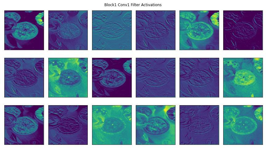
1.3 Filter Activations: Feature Maps
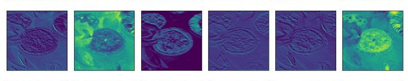
Here are some visualizations of some model layers' activations to get a better understanding of how convolutional layer filters process visual features.
We'll pass this image of an apple pie through a pre-trained CNN's convolutional blocks (i.e., groups of convolutional layers).

Below you'll see some of the outputted feature maps that the first convolutional layer activated. You'll notice that the first few convolutional layers often detect edges and geometries in the image. You can clearly make out in the activated feature maps the trace outline of our apple pie slice and the curves of the plate. These are examples of robust features.
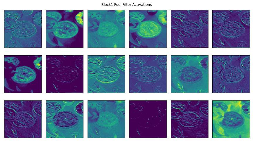
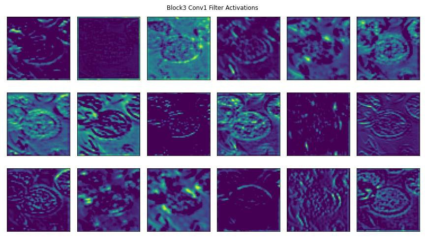
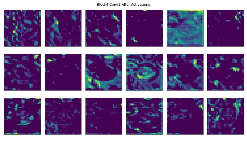
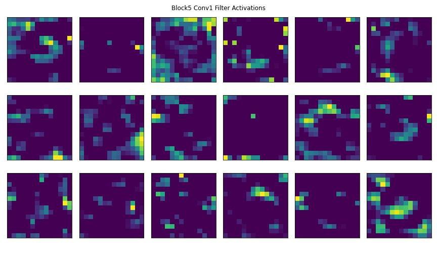
As an image passes through more convolutional layers, more precise details activate the layer's filters. In later convolutional blocks, the filter activations could be targetting pixel intensity and different splotches of color within the image. You can see some of this happening in the feature maps towards the end of the slides.
2. Activation Layers
At the end of convolution, the input image has been transformed into a stack of feature maps. Each feature map corresponds to a visual feature seen at specific locations within the input image. This feature stack's size is equal to the number of nodes (i.e., filters) in the convolutional layer.
Activation functions determine the relevancy of a given node in a neural network. A node relevant to the model's prediction will 'fire' after passing through an activation function. Regular neural networks contain these computationally-inexpensive functions. CNNs require that we use some variation of a rectified linear function (eg. ReLU).
You can think of the ReLU function as a simple maximum-value threshold function.
$$f(x)=max\{0,x\})$$
Or alternatively,
def max_thresh(val):
if val >= 0.0:
val = val
else:
val = 0.0
return valIn the above code block, the threshold is 0. The function is checking to see if any values are negative, and if so will convert them to value 0. All other values are ignored. This can be simplified even further using Numpy (see code in next section).
2a. Why ReLU?
Activation functions need to be applied to thousands of nodes at a time during the training process. Functions such as the sigmoid or hyperbolic tangent tend to prevent training due to the vanishing gradient problem, wherein high or low values of input $x$ result in no changes to the model's prediction. These functions are also computationally expensive, slowing down model training.
An important characteristic of the ReLU function is that it has a derivative function that allows for backpropagation and network convergence happens very quickly. It is computationally efficient and incredibly simple.
ReLU can be defined as:
$$ReLU'(x) = \{0, x < 0 | 1, x >= 0\}$$
Which says that nodes with negative values will have their values outputted as 0, denoting them as irrelevant for prediction. These nodes will not activate or 'fire.' Nodes with values equal to or greater than 0 will be left unchanged and will 'fire' as they're seen as relevant to making a prediction. ReLU activation layers do not change the dimensionality of the feature stack.
Here are a few lines of code to exemplify just how simple a ReLU function is:
import numpy as np
import matplotlib.pyplot as plt
x = np.random.random((3, 3)) - 0.5
print("### Matrix with Negative Values ###")
print("\n",x)
def relu(x):
return np.maximum(x, 0)
print("\n### Matrix after Rectifier Function ###")
print("\n",relu(x))### Matrix with Negative Values ###
[[ 0.18147023 0.0916844 0.35367803]
[-0.39500391 0.14322288 -0.45360101]
[-0.29513964 0.46540539 0.14467363]]
### Matrix after Rectifier Function ###
[[0.18147023 0.0916844 0.35367803]
[0. 0.14322288 0. ]
[0. 0.46540539 0.14467363]]As we can see, previous negative values in our matrix x have been passed through an argmax function, with a threshold of 0. This is what occurs en-masse for the nodes in our convolutional layers to determine which node will 'fire.'
3. Pooling Layers
Recall that convolutional layers are a stack of visual feature maps. As the complexity of a dataset increases, so must the number of filters in the convolutional layers. Each filter is being tasked with the job of identifying different visual features in the image. As we increase the number of feature maps in the stack, we increase the dimensionality, parameters, and the possibility of overfitting.
To account for this, CNNs have Pooling layers after the convolutional layers. Pooling layers take the stack of feature maps as an input and perform down-sampling. In this tutorial, two types of pooling layers will be introduced.
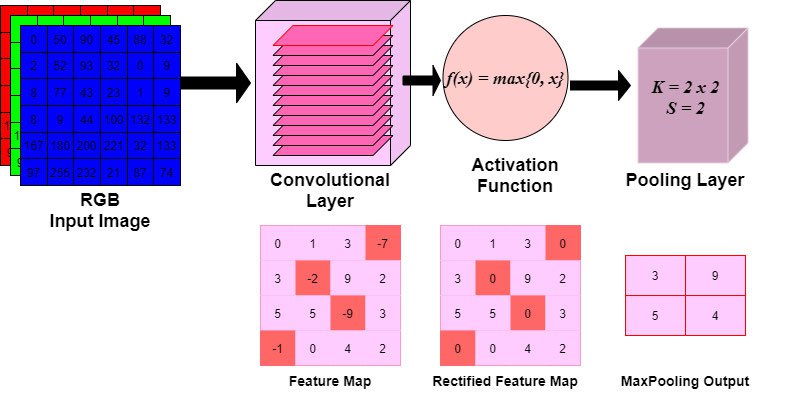
3.1 Max Pooling Layers:
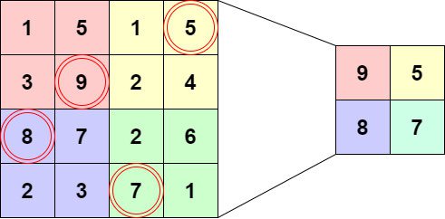
MaxPooling layers take two input arguments: kernel width and height, and stride. The kernel starts at the top left corner of a feature map, then passes over the pixels to the right at the defined stride. The pixel with the highest value contained in the kernel window will be used as the value for the corresponding node in the pooling layer.
In the below example, we have a single feature map. Our pooling layers have the following arguments:
Kernel Size: 2 x 2
Stride: 2
As the kernel slides across the feature map at a stride of 2, the maximum values contained in the window are connected to the nodes in the pooling layer. As you can see, the dimension of the feature map is reduced by half.
This process occurs for all feature maps in the stack, so the number of feature maps will remain the same. The only change is each feature map's dimensions.
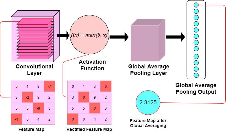
3.2 Global Average Pooling Layer:
With Global Averaging, the feature maps' dimensions are reduced drastically by transforming the 3-Dimensional feature stack into a 1-Dimensional vector.
The values of all pixels are averaged and outputted to a single node in a 1-Dimensional vector. This results in the dimensions $(,K)$ where $K$ is the total number of feature maps.
In the below graphic, we've employed a Global Average Pooling layer to reduce our example feature map's dimensionality. Note how the feature map is passed through a ReLU activation function before having its values averaged and outputted as a single node.
You will often find that Max Pooling is used the most for image classification. This decision runs off the assumption that visual features of interest will tend to have higher pixel values, and Max Pooling can detect these features while maintaining spatial arrangements.
This is not to say that Global Average Pooling is never used. Because Global Average Pooling results in a single vector of nodes, some powerful CNNs utilize this approach for flattening their 3-Dimensional feature stacks.
4. The Fully-Connected Layer
Recall that Fully-Connected Neural Networks are constructed out of layers of nodes, wherein each node is connected to all other nodes in the previous layer. This type of network is placed at the end of our CNN architecture to make a prediction, given our learned, convolved features.
The goal of the Fully-Connected layer is to make class predictions. The Fully-Connected layer will take as input a flattened vector of nodes that have been activated in the previous Convolutional layers. The vector input will pass through two to three — sometimes more — dense layers and pass through a final activation function before being sent to the output layer. The activation function used for prediction does not need to be a rectified linear unit. Selecting the right activation function depends on the type of classification problem, and two common functions are:
- Sigmoid is generally used for binary classification problems, as it is a logistic function
- Softmax ensures that the sum of values in the output layer sum to 1 and can be used for both binary and multi-class classification problems.
The final output vector size should be equal to the number of classes you are predicting, just like in a regular neural network.
Implementation of a CNN in Keras
Downloading and preparing the dataset
The next two lines will run some console commands to extract the Food-101 dataset and download it to your local machine. If you wish to download it to a specific directory, cd to that directory first before running the next two commands.
This may take 5 to 10 minutes, so maybe make yourself a cup of coffee!
!wget http://data.vision.ee.ethz.ch/cvl/food-101.tar.gz!tar xzvf food-101.tar.gzBefore we explore the image data further, you should divide the dataset into training and validation subsets.
The food-101 dataset also includes some .meta files which have already indexed images as 'train' or 'test' data. These files split the dataset 75/25 for training and testing and can be found in food-101/meta/train.json and food-101/meta/test.json.
In the following split_dataset function, we are using the provided meta files to split the images into train and test directories. The meta files are loaded as dictionaries, where the food name is the key, and a list of image paths are the values. Using shutil, we can use these paths to move the images to the train/test directories:
# Move data from images to images/train or images/test:
import shutil
from collections import defaultdict
import json
from pathlib import Path
import os
def split_dataset(root_food_path):
"""Takes in the path for food-101 directory and creates train/test dirs of images"""
data_paths = {
'train': root_food_path/'meta/train.json',
'test': root_food_path/'meta/test.json'
}
for data_type, meta_path in data_paths.items():
# Make the train/test dirs
os.makedirs(root_food_path/data_type, exist_ok=True)
# Read the meta files.
# These are loaded as a dict of food names with a list of image paths
# E.g. {"<food_name>": ["<food_name>/<image_num>", ...], ...}
food_images = json.load(open(meta_path, 'r'))
for food_name, image_paths in food_images.items():
# Make food dir in train/test dir
os.makedirs(root_food_path/data_type/food_name, exist_ok=True)
# Move images from food-101/images to food-101/train (or test)
for image_path in image_paths:
image_path = image_path + '.jpg'
shutil.move(root_food_path/'images'/image_path, root_food_path/data_type/image_path)Below, we're running the function we just defined. Make sure to specify download_dir as the directory you downloaded the food dataset to. The download_dir variable will be used many times in the subsequent functions.
from pathlib import Path
download_dir = Path('<your directory here>')
split_dataset(download_dir/'food-101')Our directory structure should look like this now:
food-101
├───test
│ ├───apple_pie
│ │ ├───134.jpg
│ │ ...
│ ...
│ └───waffles
│ ├───6312.jpg
│ ...
└───train
├───apple_pie
│ ├───134.jpg
│ ...
...
└───waffles
├───6312.jpg
...Preprocessing Image Data
Recall how images are interpreted by a computer. A computer's vision does not see an apple pie image like we do; instead it sees a three-Dimensional array of values ranging from 0 to 255.
Before we can train a model to recognize images, the data needs to be prepared in a certain way. Depending on the computer vision task, some preprocessing steps may not need to be implemented, but you will almost always need to perform normalization and augmentation.
1. Normalization
It is best practice to normalize your input images' range of values prior to feeding them into your model. In our preprocessing step, we'll use the rescale parameter to rescale all the numerical values in our images to a value in the range of 0 to 1.
This is very important since some images might have very high pixel values while others have lower pixel values. When you rescale all images, you ensure that each image contributes to the model's loss function evenly.
In other words, rescaling the image data ensures that all images are considered equally when the model is training and updating its weights.
2. Augmentation
Classification of images with objects is required to be statistically invariant. Recall that all images are represented as three-dimensional arrays of pixel values, so an apple pie in the center of an image appears as a unique array of numbers to the computer. However, we need to consider the very-likely chance that not all apple pie images will appear the same.
We want to train our algorithm to be invariant to improve its ability to generalize the image data. This can be done by introducing augmentations into the preprocessing steps. Augmentations increase the variance of the training data in a variety of ways, including: random rotation, increase/decreasing brightness, shifting object positions, and horizontally/vertically flipping images.
For this classification task, we're going to augment the image data using Keras' ImageDataGenerator class. You'll see below how introducing augmentations into the data transforms a single image into similar - but altered - images of the same food. This is useful if we want our algorithm to recognize our food from different angles, brightness levels, or positions.
import numpy as np
from keras.preprocessing.image import ImageDataGenerator
# Image augmentations
example_generator = ImageDataGenerator(
rescale=1 / 255., # normalize pixel values between 0-1
vertical_flip=True, # vertical transposition
horizontal_flip=True, # horizontal transposition
rotation_range=90, # random rotation at 90 degrees
height_shift_range=0.3, # shift the height of the image 30%
brightness_range=[0.1, 0.9] # specify the range in which to decrease/increase brightness
)
As you can see, our original apple pie image has been augmented such that our algorithm will be exposed to various apple pie images that have either been rotated, shifted, transposed, darkened or a combination of the four.
Augmentation is beneficial when working with a small dataset, as it increases variance across images. We only apply image augmentations for training. We never apply these transformations when we are testing. We want to measure the performance of the CNN's ability to predict real-world images that it was not previously exposed to.
Using ImageDataGenerator for training
Like in the example above, now we will apply multiple augmentations to our training data for all images. ImageDataGenerator lets us easily load batches of data for training using the flow_from_directory method. Our directories holding the training and testing data are structured perfectly for this method, which requires the input images to be housed in subdirectories corresponding to their class label.
We specify a validation split with the validation_split parameter, which defines how to split the data during the training process. At the end of each epoch, a prediction will be made on a small validation subset to inform us of how well the model is training.
from keras.preprocessing.image import ImageDataGenerator
train_generator = ImageDataGenerator(
rescale=1/255., # normalize pixel values between 0-1
brightness_range=[0.1, 0.7], # specify the range in which to decrease/increase brightness
width_shift_range=0.5, # shift the width of the image 50%
rotation_range=90, # random rotation by 90 degrees
horizontal_flip=True, # 180 degree flip horizontally
vertical_flip=True, # 180 degree flip vertically
validation_split=0.15 # 15% of the data will be used for validation at end of each epoch
)Our dataset is quite large, and although CNNs can handle high dimensional inputs such as images, processing, and training can still take quite a long time. For this tutorial, we'll load only certain class labels from the image generators. Our CNN will have an output layer of 10 nodes corresponding to the first 10 classes in the directory.
import os
class_subset = sorted(os.listdir(download_dir/'food-101/images'))[:10]When we call the flow_from_directory method from our generators, we provide the target_size - which resizes our input images. Typically, images are resized to square dimensions such as 32x32 or 64x64. Some powerful CNNs take input images with the dimensions of 224x224. For this tutorial, we'll resize our images to 128x128. Not too small that important information is lost to the low-resolution, but also not too high so that our simple CNN's performance is slowed down.
BATCH_SIZE = 32
traingen = train_generator.flow_from_directory(download_dir/'food-101/train',
target_size=(128, 128),
batch_size=BATCH_SIZE,
class_mode='categorical',
classes=class_subset,
subset='training',
shuffle=True,
seed=42)
validgen = train_generator.flow_from_directory(download_dir/'food-101/test',
target_size=(128, 128),
batch_size=BATCH_SIZE,
class_mode='categorical',
classes=class_subset,
subset='validation',
shuffle=True,
seed=42)Found 6380 images belonging to 10 classes.
Found 370 images belonging to 10 classes.Note
Check if Keras is using your GPU. The following function call will output True if Keras is using your GPU for training.
python import tensorflow as tf tf.test.is_gpu_available()
Alternatively, specifically check for GPU's with cuda support: python tf.test.is_gpu_available(cuda_only=True)
CNN Architecture in Keras
Keras allows you to build simple CNNs in just a few lines of code. In this section, we'll create a CNN with all the essential building blocks:
- the Input Layer
- the Convolutional Layers
- the Fully-Connected Layer
For this tutorial, we'll be creating a Keras Model with the Sequential model API. A Sequential instance, which we'll define as a variable called model in our code below, is a straightforward approach to defining a neural network model with Keras.
As the name suggests, this instance will allow you to add the different layers of your model and connect them sequentially. Sequential models take an input volume, in our case an image, and pass this volume through the added layers in a sequence. This API is limited to single-inputs and single-outputs. The order in which you add the layers to this model is the sequence that inputted data will pass through.
We'll add our Convolutional, Pooling, and Dense layers in the sequence that we want out data to pass through in the code block below.
For more information on this class, you can always read the docs.
Dropout
A form of regularization, called Dropout, will also be employed. Dropout was proposed by Srivastava, et al. in a 2014 paper titled Dropout: A Simple Way to Prevent Neural Networks from Overfitting. As the title states, dropout is a technique employed to help prevent over-fitting. When we introduce this regularization, we randomly select neurons to be ignored during training. This removes contributions to the activation of neurons temporarily, and the weight updates that would occur during backpropagation are also not applied. This improves the model's generalization and prevents certain sets of weights from specializing in specific features, which could lead to overfitting if not constrained.
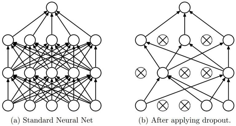
Dropout layers in Keras randomly select nodes to be ignored, given a probability as an argument. In the following CNN, dropout will be added at the end of each convolutional block and in the fully-connected layer.
Writing our Model in Keras
Finally! We're ready to create a basic CNN using Keras.
Below is a relatively simplistic architecture for our first CNN. Let's go over some details before we train the model:
- We will have four convolutional 'blocks' comprised of (a) Convolutional layers, (b) a Max Pooling layer, and (c) Dropout regularization.
- Each Convolutional layer will have a Stride of one (1), the default setting for the
Conv2Dmethod. - Activation layers are defined in the
Conv2Dmethod, and as discussed before, will be using a rectified linear unit (ReLU). - All Convolutional blocks will use a filter window size of 3x3, except the final convolutional block, which uses a window size of 5x5.
- All Convolutional blocks will also make use of the
activationparameter - ReLU will be used as an argument. - We call the
Flatten()method at the start of the Fully-Connected Layer. This is to transform the 3-Dimensional feature maps into a 1-Dimensional input tensor. - We'll construct a Fully-Connected layer using
Denselayers. - Since this is a multi-class problem, our Fully-Connected layer has a Softmax activation function.
Note
Use this to clear the model if you test different parameters python tf.keras.backend.clear_session()
from keras.models import Sequential
from keras.layers import Conv2D, MaxPooling2D, Flatten, Dense, Dropout, Activation
from keras.regularizers import l1_l2
model = Sequential()
#### Input Layer ####
model.add(Conv2D(filters=32, kernel_size=(3,3), padding='same',
activation='relu', input_shape=(128, 128, 3)))
#### Convolutional Layers ####
model.add(Conv2D(32, (3,3), activation='relu'))
model.add(MaxPooling2D((2,2))) # Pooling
model.add(Dropout(0.2)) # Dropout
model.add(Conv2D(64, (3,3), padding='same', activation='relu'))
model.add(Conv2D(64, (3,3), activation='relu'))
model.add(MaxPooling2D((2,2)))
model.add(Dropout(0.2))
model.add(Conv2D(128, (3,3), padding='same', activation='relu'))
model.add(Conv2D(128, (3,3), activation='relu'))
model.add(Activation('relu'))
model.add(MaxPooling2D((2,2)))
model.add(Dropout(0.2))
model.add(Conv2D(512, (5,5), padding='same', activation='relu'))
model.add(Conv2D(512, (5,5), activation='relu'))
model.add(MaxPooling2D((4,4)))
model.add(Dropout(0.2))
#### Fully-Connected Layer ####
model.add(Flatten())
model.add(Dense(1024, activation='relu'))
model.add(Dropout(0.2))
model.add(Dense(len(class_subset), activation='softmax'))
model.summary() # a handy way to inspect the architectureModel: "sequential"
_________________________________________________________________
Layer (type) Output Shape Param #
=================================================================
conv2d (Conv2D) (None, 128, 128, 32) 896
_________________________________________________________________
conv2d_1 (Conv2D) (None, 126, 126, 32) 9248
_________________________________________________________________
max_pooling2d (MaxPooling2D) (None, 63, 63, 32) 0
_________________________________________________________________
dropout (Dropout) (None, 63, 63, 32) 0
_________________________________________________________________
conv2d_2 (Conv2D) (None, 63, 63, 64) 18496
_________________________________________________________________
conv2d_3 (Conv2D) (None, 61, 61, 64) 36928
_________________________________________________________________
max_pooling2d_1 (MaxPooling2 (None, 30, 30, 64) 0
_________________________________________________________________
dropout_1 (Dropout) (None, 30, 30, 64) 0
_________________________________________________________________
conv2d_4 (Conv2D) (None, 30, 30, 128) 73856
_________________________________________________________________
conv2d_5 (Conv2D) (None, 28, 28, 128) 147584
_________________________________________________________________
activation (Activation) (None, 28, 28, 128) 0
_________________________________________________________________
max_pooling2d_2 (MaxPooling2 (None, 14, 14, 128) 0
_________________________________________________________________
dropout_2 (Dropout) (None, 14, 14, 128) 0
_________________________________________________________________
conv2d_6 (Conv2D) (None, 14, 14, 512) 1638912
_________________________________________________________________
conv2d_7 (Conv2D) (None, 10, 10, 512) 6554112
_________________________________________________________________
max_pooling2d_3 (MaxPooling2 (None, 2, 2, 512) 0
_________________________________________________________________
dropout_3 (Dropout) (None, 2, 2, 512) 0
_________________________________________________________________
flatten (Flatten) (None, 2048) 0
_________________________________________________________________
dense (Dense) (None, 1024) 2098176
_________________________________________________________________
dropout_4 (Dropout) (None, 1024) 0
_________________________________________________________________
dense_1 (Dense) (None, 10) 10250
=================================================================
Total params: 10,588,458
Trainable params: 10,588,458
Non-trainable params: 0
_________________________________________________________________Notes on Training: Callbacks
Keras models include the ability to interact automatically with the model during training. We're going to use a few callback techniques
EarlyStopping- monitors the performance of the model and stopping the training process prevents overtrainingModelCheckpoint- saves the best weights for the model to a file after each epochPlotLossesKeras- from the _livelossplot_ library, shows graphs of loss and accuracy and updates after each epoch
The Early Stopping used here will monitor the validation loss and ensure that it is decreasing. If we were monitoring validation accuracy, we would be monitoring for an increase in the metric. A delay is also used to ensure that Early Stopping is not triggered at the first sign of validation loss not decreasing. We use the 'patience' parameter to invoke this delay. In summary:
- Early Stopping monitors a performance metric to prevent overtraining
- the monitor parameter is set to
val_loss. This callback will monitor the validation loss at the end of each epoch - the mode parameter is set to
minsince we are seeking to minimize the validation loss - the patience parameter specifies how long a delay before halting the training process
- this model will train for a maximum of 100 epochs, however, if the validation loss does not decrease for 10 consecutive epochs - the training will halt
Finally, instead of PlotLossesKeras you can use the built-in Tensorboard callback as well. Instead of plotting in this notebook, you'll have to run a terminal command to launch Tensorboard on localhost. This will provide a lot more information and flexibility than the plots from PlotLossesKeras.
%%time
from keras.optimizers import RMSprop
from keras.callbacks import ModelCheckpoint, EarlyStopping, TensorBoard
from livelossplot import PlotLossesKeras
steps_per_epoch = traingen.samples // BATCH_SIZE
val_steps = validgen.samples // BATCH_SIZE
n_epochs = 100
optimizer = RMSprop(learning_rate=0.0001)
model.compile(loss='categorical_crossentropy', optimizer=optimizer, metrics=['accuracy'])
# Saves Keras model after each epoch
checkpointer = ModelCheckpoint(filepath='img_model.weights.best.hdf5',
verbose=1,
save_best_only=True)
# Early stopping to prevent overtraining and to ensure decreasing validation loss
early_stop = EarlyStopping(monitor='val_loss',
patience=10,
restore_best_weights=True,
mode='min')
# tensorboard_callback = TensorBoard(log_dir="./logs")
# Actual fitting of the model
history = model.fit(traingen,
epochs=n_epochs,
steps_per_epoch=steps_per_epoch,
validation_data=validgen,
validation_steps=val_steps,
callbacks=[early_stop, checkpointer, PlotLossesKeras()],
verbose=False)
accuracy
training (min: 0.118, max: 0.552, cur: 0.548)
validation (min: 0.114, max: 0.599, cur: 0.599)
Loss
training (min: 1.269, max: 2.286, cur: 1.270)
validation (min: 1.209, max: 2.267, cur: 1.252)
Wall time: 45min 6sYou'll notice that the plot will update after each epoch thanks to the PlotLossesKeras callback.
Furthermore, you can see that this particular model took about 45 minutes to train on an NVIDIA 1080 Ti GPU. Remember that this was only for 10 of the food classes. If we increase that to all 101 food classes, this model could take 20+ hours to train.
Evaluating Our Network
We'll now evaluate the model's predictive ability on the testing data. To do so, you must define an image generator for the testing data. This generator will not apply any image augmentations - as this is supposed to represent a real-world scenario in which a new image is introduced to the CNN for prediction. The only argument we need for this test generator is the normalization parameter - rescale.
We also do not need to specify the same batch size when we pull data from the directory. A batch size of 1 will suffice.
Note that the images are being resized to 128x128 dimensions and that we are specifying the same class subsets as before.
test_generator = ImageDataGenerator(rescale=1/255.)
testgen = test_generator.flow_from_directory(download_dir/'food-101/test',
target_size=(128, 128),
batch_size=1,
class_mode=None,
classes=class_subset,
shuffle=False,
seed=42)Found 2500 images belonging to 10 classes.model.load_weights('img_model.weights.best.hdf5')
predicted_classes = model.predict_classes(testgen)
class_indices = traingen.class_indices
class_indices = dict((v,k) for k,v in class_indices.items())
true_classes = testgen.classesAbove, we load the weights that achieved the best validation loss during training. We use the model's predict_classes method, which will return the predicted class label's index value.
Below, we'll define a few functions to help display our model's predictive performance.
display_results() will compare the images' true labels with the predicted labels.
plot_predictions() will allow us to visualize a sample of the test images, and the labels that the model generates.
import pandas as pd
import matplotlib.pyplot as plt
from sklearn.metrics import precision_recall_fscore_support, accuracy_score
def display_results(y_true, y_preds, class_labels):
results = pd.DataFrame(precision_recall_fscore_support(y_true, y_preds),
columns=class_labels).T
results.rename(columns={0: 'Precision', 1: 'Recall',
2: 'F-Score', 3: 'Support'}, inplace=True)
results.sort_values(by='F-Score', ascending=False, inplace=True)
global_acc = accuracy_score(y_true, y_preds)
print("Overall Categorical Accuracy: {:.2f}%".format(global_acc*100))
return results
def plot_predictions(y_true, y_preds, test_generator, class_indices):
fig = plt.figure(figsize=(20, 10))
for i, idx in enumerate(np.random.choice(test_generator.samples, size=20, replace=False)):
ax = fig.add_subplot(4, 5, i + 1, xticks=[], yticks=[])
ax.imshow(np.squeeze(test_generator[idx]))
pred_idx = y_preds[idx]
true_idx = y_true[idx]
plt.tight_layout()
ax.set_title("{}\n({})".format(class_indices[pred_idx], class_indices[true_idx]),
color=("green" if pred_idx == true_idx else "red"))plot_predictions(true_classes, predicted_classes, testgen, class_indices)
Fig 15. Each image has its predicted class label as a title, and its true class label is formatted in parentheses
display_results(true_classes, predicted_classes, class_indices.values())Overall Categorical Accuracy: 56.96%| Precision | Recall | F-Score | Support | |
|---|---|---|---|---|
| beef_carpaccio | 0.804545 | 0.708 | 0.753191 | 250.0 |
| bibimbap | 0.719008 | 0.696 | 0.707317 | 250.0 |
| beet_salad | 0.679842 | 0.688 | 0.683897 | 250.0 |
| beignets | 0.524510 | 0.856 | 0.650456 | 250.0 |
| baby_back_ribs | 0.463675 | 0.868 | 0.604457 | 250.0 |
| beef_tartare | 0.586777 | 0.568 | 0.577236 | 250.0 |
| baklava | 0.594286 | 0.416 | 0.489412 | 250.0 |
| breakfast_burrito | 0.474178 | 0.404 | 0.436285 | 250.0 |
| bread_pudding | 0.453988 | 0.296 | 0.358354 | 250.0 |
| apple_pie | 0.422414 | 0.196 | 0.267760 | 250.0 |
Our model has achieved an Overall Accuracy of < 60%, which fluctuates every training session. This is far from high performance, but for a simple CNN written from scratch, this can be expected!
We can see the class-wise precision and recall using our display_results() function. The output dataframe is sorted by highest F-Score, which is the balanced mean between precision and recall.
It seems the model is performing well at classifying some food images while struggling to recognize others. Using the returned metrics, we can make some concluding statements on the model's performance:
- The model predicts a large portion of the images as baby_back_ribs, which results in a high recall (> 95%!) for this particular class but sacrifices precision.
- The model can identify images of beignets, bibimbap, beef_carpaccio & beet_salad moderately well, with F-scores between ~0.60 - 0.80
- The model did not perform well for apple_pie in particular - this class ranked the lowest in terms of recall.
Conclusion
In this article, you were introduced to the essential building blocks of Convolutional Neural Networks and some strategies for regularization. Feel free to copy the architecture defined in this article and make your own adjustments accordingly. It should provide you with a general understanding of CNNs, and a decently-performing starter model. Try experimenting with adding/removing convolutional layers and adjusting the dropout or learning rates to see how this impacts performance! And of course, always be sure to Read the Docs if this is your first time using Keras!
What's Next?
You will find that oftentimes many data scientists do not actually write their own networks from scratch, as we've done here. Advancements in the field of Deep Learning has produced some amazing models for Computer Vision tasks! These models are also not privy to a select few. Through an awesome technique called Transfer Learning, you can easily load one of these models and modify them according to your own dataset! Check out our article on Transfer Learning here!
Meet the Authors

James is a data science consultant and technical writer. He has spent four years working on data-driven projects and delivering machine learning solutions in the research industry.