
Data Science Consultant
Hands-on Transfer Learning with Keras and the VGG16 Model
LearnDataSci is reader-supported. When you purchase through links on our site, earned commissions help support our team of writers, researchers, and designers at no extra cost to you.
In a previous article, we introduced the fundamentals of image classification with Keras, where we built a CNN to classify food images. Our model didn't perform that well, but we can make significant improvements in accuracy without much more training time by using a concept called Transfer Learning.
By the end of this article, you should be able to:
- Download a pre-trained model from Keras for Transfer Learning
- Fine-tune the pre-trained model on a custom dataset
Let's get started.
What Is Transfer Learning?
In the previous article, we defined our own Convolutional Neural Network and trained it on a food image dataset. We saw that the performance of this from-scratch model was drastically limited.
This model had to first learn how to detect generic features in the images, such as edges and blobs of color, before detecting more complex features.
In real-world applications, this can take days of training and millions of images to achieve high performance. It would be easier for us to download a generic pretrained model and retrain it on our own dataset. This is what Transfer Learning entails.
In this way, Transfer Learning is an approach where we use one model trained on a machine learning task and reuse it as a starting point for a different job. Multiple deep learning domains use this approach, including Image Classification, Natural Language Processing, and even Gaming! The ability to adapt a trained model to another task is incredibly valuable.
CNN Review
This tutorial expects that you have an understanding of Convolutional Neural Networks. If you want an in-depth look into these networks, feel free to read our previous article.
In this section, we'll review CNN building blocks. Feel free to skip ahead for the Python implementation.
Convolutional Neural Network Architecture
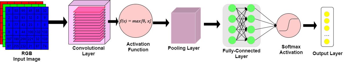
Recall that CNN architecture contains some essential building blocks such as:
1. Convolutional Layer:
- Conv. Layers will compute the output of nodes that are connected to local regions of the input matrix.
- Dot products are calculated between a set of weights (commonly called a filter) and the values associated with a local region of the input.
2. ReLu (Activation) Layer:
- The output volume of the Conv. Layer is fed to an elementwise activation function, commonly a Rectified-Linear Unit (ReLu).
- The ReLu layer will determine whether an input node will 'fire' given the input data. This 'firing' signals whether the convolution layer's filters have detected a visual feature.
- A ReLu function will apply a $max(0,x)$ function, thresholding at 0.
- The dimensions of the volume are left unchanged.
3. Pooling Layer:
- A down-sampling strategy is applied to reduce the width and height of the output volume.
4. Fully-Connected Layer:
- The output volume, i.e. 'convolved features', are passed to a Fully-Connected Layer of nodes.
- Like conventional neural-networks, every node in this layer is connected to every node in the volume of features being fed-forward.
- The class probabilities are computed and are outputted in a 3D array (the Output Layer) with dimensions:
[1 x 1 x K], where K is the number of classes.
Writing these types of models from scratch can be incredibly tricky, especially if we don't have a dataset of sufficient size. The CNN model that we'll discuss later in this article has been pre-trained on millions of photos! We'll explore how we can use the pre-trained architecture to solve our custom classification problem.
Predicting Food Labels with a Keras CNN
Initially, we wrote a simple CNN from scratch. We'll load the same model as before to generate some predictions and calculate its accuracy, which will be used to compare the performance of the new model using Transfer Learning.
"""Load the written-from-scratch cnn"""
from keras.models import load_model
scratch_model = load_model('scratch_img_model.hdf5')
scratch_model.summary()Model: "sequential"
_________________________________________________________________
Layer (type) Output Shape Param #
=================================================================
conv2d (Conv2D) (None, 128, 128, 32) 896
_________________________________________________________________
conv2d_1 (Conv2D) (None, 126, 126, 32) 9248
_________________________________________________________________
max_pooling2d (MaxPooling2D) (None, 63, 63, 32) 0
_________________________________________________________________
dropout (Dropout) (None, 63, 63, 32) 0
_________________________________________________________________
conv2d_2 (Conv2D) (None, 63, 63, 64) 18496
_________________________________________________________________
conv2d_3 (Conv2D) (None, 61, 61, 64) 36928
_________________________________________________________________
max_pooling2d_1 (MaxPooling2 (None, 30, 30, 64) 0
_________________________________________________________________
dropout_1 (Dropout) (None, 30, 30, 64) 0
_________________________________________________________________
conv2d_4 (Conv2D) (None, 30, 30, 128) 73856
_________________________________________________________________
conv2d_5 (Conv2D) (None, 28, 28, 128) 147584
_________________________________________________________________
activation (Activation) (None, 28, 28, 128) 0
_________________________________________________________________
max_pooling2d_2 (MaxPooling2 (None, 14, 14, 128) 0
_________________________________________________________________
dropout_2 (Dropout) (None, 14, 14, 128) 0
_________________________________________________________________
conv2d_6 (Conv2D) (None, 14, 14, 512) 1638912
_________________________________________________________________
conv2d_7 (Conv2D) (None, 10, 10, 512) 6554112
_________________________________________________________________
max_pooling2d_3 (MaxPooling2 (None, 2, 2, 512) 0
_________________________________________________________________
dropout_3 (Dropout) (None, 2, 2, 512) 0
_________________________________________________________________
flatten (Flatten) (None, 2048) 0
_________________________________________________________________
dense (Dense) (None, 1024) 2098176
_________________________________________________________________
dropout_4 (Dropout) (None, 1024) 0
_________________________________________________________________
dense_1 (Dense) (None, 10) 10250
=================================================================
Total params: 10,588,458
Trainable params: 10,588,458
Non-trainable params: 0
_________________________________________________________________Our from-scratch CNN has a relatively simple architecture: 7 convolutional layers, followed by a single densely-connected layer.
Using the old CNN to calculate an accuracy score (details of which you can find in the previous article) we found that we had an accuracy score of ~58%.
With such an accuracy score, the from-scratch CNN performs moderately well, at best. We could improve the accuracy with a sufficiently-sized training dataset, which we do not have.
In practice, you should write a CNN from scratch only if you have a large dataset. In this tutorial, we'll download a pretrained model and re-train it on our own dataset to generate a better model.
How Does Transfer Learning Work?
Transfer Learning partially resolves the limitations of the isolated learning paradigm:
"The current dominant paradigm for ML is to run an ML algorithm on a given dataset to generate a model. The model is then applied in real-life tasks. We call this paradigm isolated learning because it does not consider any other related information or the knowledge learned in the past." (Liu, 2016)
Transfer Learning gives us the ability to share learned features across different learning tasks.
Domains and Tasks
We can understand Transfer Learning in terms of Domains and Tasks. In our case, the domain is image classification, and our task is to classify food images. Like we did previously, starting from scratch would require many optimizations, more data, and longer training to improve performance. If we use a CNN that's already been optimized and trained for a similar domain and task, we could convert it to work with our task. This is what transfer learning accomplishes.
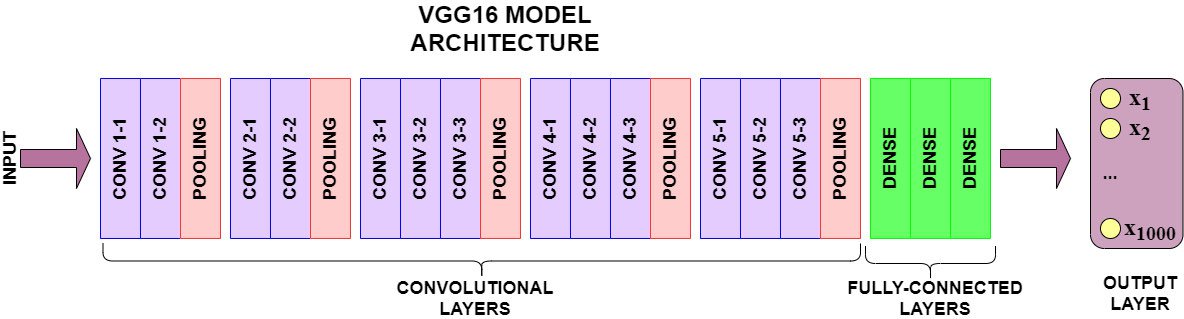
We will utilize the pre-trained VGG16 model, which is a convolutional neural network trained on 1.2 million images to classify 1000 different categories. Since the domain and task for VGG16 are similar to our domain and task, we can use its pre-trained network to do the job.
For details on a more mathematical definition, see the paper Improving EEG-Based Emotion Classification Using Conditional Transfer Learning.
Using Pretrained Convolutional Layers
Our Transfer Learning approach will involve using layers that have been pre-trained on a source task to solve a target task. We would typically download some pre-trained model and "cut off" its top portion (the fully-connected layer), leaving us with only the convolutional and pooling layers.
Using the pre-trained layers, we'll extract visual features from our target task/dataset.
When using these pre-trained layers, we can decide to freeze specific layers from training. We'll be using the pre-trained weights as-they-come and not updating them with backpropagation.
Alternatively, we can freeze most of the pre-trained layers but allow other layers to update their weights to improve target data classification.
How to Utilize the VGG16 Model
VGG16 is a convolutional neural network trained on a subset of the ImageNet dataset, a collection of over 14 million images belonging to 22,000 categories. K. Simonyan and A. Zisserman proposed this model in the 2015 paper, Very Deep Convolutional Networks for Large-Scale Image Recognition.
In the 2014 ImageNet Classification Challenge, VGG16 achieved a 92.7% classification accuracy. But more importantly, it has been trained on millions of images. Its pre-trained architecture can detect generic visual features present in our Food dataset.
Now suppose we have many images of two kinds of cars: Ferrari sports cars and Audi passenger cars. We want to generate a model that can classify an image as one of the two classes. Writing our own CNN is not an option since we do not have a dataset sufficient in size. Here's where Transfer Learning comes to the rescue!
We know that the ImageNet dataset contains images of different vehicles (sports cars, pick-up trucks, minivans, etc.). We can import a model that has been pre-trained on the ImageNet dataset and use its pre-trained layers for feature extraction.
Now we can't use the entirety of the pre-trained model's architecture. The Fully-Connected layer generates 1,000 different output labels, whereas our Target Dataset has only two classes for prediction. So we'll import a pre-trained model like VGG16, but "cut off" the Fully-Connected layer - also called the "top" model.
Once the pre-trainedlayers have been imported, excluding the "top" of the model, we can take 1 of 2 Transfer Learning approaches.
1. Feature Extraction Approach
We use the pre-trained model's architecture to create a new dataset from our input images in this approach. We'll import the Convolutional and Pooling layers but leave out the "top portion" of the model (the Fully-Connected layer).
Recall that our example model, VGG16, has been trained on millions of images - including vehicle images. Its convolutional layers and trained weights can detect generic features such as edges, colors, wheels, windshields, etc.
We'll pass our images through VGG16's convolutional layers, which will output a Feature Stack of the detected visual features. From here, it's easy to flatten the 3-Dimensional feature stack into a NumPy array - ready for whatever modeling you'd prefer to conduct.
We can do feature extraction in the following manner:
- Download the pre-trained model. Ensure that the "top" portion of the model - the Fully-Connected layer - is not included.
- Pass the image data through the pre-trained layers to extract convolved visual features
- The outputted feature stack will be 3-Dimensional, and for it to be used for prediction by other machine learning classifiers, it will need to be flattened.
- At this point, you have two options:
- Stand-Alone Extractor: In this scenario, you can use the pre-trained layers to extract image features once. The extracted features would then create a new dataset that doesn't require any image processing.
- Bootstrap Extractor: Write your own Fully-Connected layer, and integrate it with the pre-trained layers. In this sense, you are bootstrapping your own "top model" onto the pre-trained layers. Initialize this Fully-Connected layer with random weights, which will update via backpropagation during training.
This article will show how to implement a "bootstrapped" extraction of image data with the VGG16 CNN. Pre-trained layers will convolve the image data according to ImageNet weights. We will bootstrap a Fully-Connected layer to generate predictions.
2. Fine-Tuning Approach
In this approach, we employ a strategy called Fine-Tuning. The goal of fine-tuning is to allow a portion of the pre-trained layers to retrain.
In the previous approach, we used the pre-trained layers of VGG16 to extract features. We passed our image dataset through the convolutional layers and weights, outputting the transformed visual features. There was no actual training on these pre-trained layers.
Fine-tuning a Pre-trained Model entails:
- Bootstrapping a new "top" portion of the model (i.e., Fully-Connected and Output layers)
- Freezing pre-trained convolutional layers
- Un-freezing the last few pre-trained layers training.
The frozen pre-trained layers will convolve visual features as usual. The non-frozen (i.e., the 'trainable') pre-trained layers will be trained on our custom dataset and update according to the Fully-Connected layer's predictions.
In this article, we will demonstrate how to implement Fine-tuning on the VGG16 CNN. We will load some of the pre-trained layers as 'trainable', pass image data through the pre-trained layers, and 'fine-tune' the trainable layers alongside our Fully-Connected layer.
Downloading the Dataset
Before we demonstrate either of these approaches, ensure you've downloaded the data for this tutorial.
To access the data used in this tutorial, check out the Image Classification with Keras article. You can find the terminal commands and functions for splitting the data in this section. If you're starting from scratch, make sure to run the split_dataset function after downloading the dataset so that the images are in the correct directories for this tutorial.
Using Transfer Learning for Food Classification
Pre-trained models, such as VGG16, are easily downloaded using the Keras API. We'll go ahead and use VGG16 for the tutorial, but you should explore the other models available! Many of them have been trained on the ImageNet dataset and come with their advantages and disadvantages. You can find a list of the available models here.
We've also imported something called a preprocess_function alongside the VGG16 model. Recall that image data must be normalized before training. Images are composed of 3-Dimensional matrices containing numerical values in a range of [0, 255]. Not all CNNs have the same normalization scheme, however.
The VGG16 model was trained on data wherein pixel values ranged from [0, 255], and the mean pixel values of the dataset are subtracted from each image channel.
Other models have different normalization schemes, details of which are in their documentation. Some models require scaling the numerical values to be between (-1, +1).
Preparing the training and testing data
Let's first import some necessary libraries.
import os
from keras.models import Model
from keras.optimizers import Adam
from keras.applications.vgg16 import VGG16, preprocess_input
from keras.preprocessing.image import ImageDataGenerator
from keras.callbacks import ModelCheckpoint, EarlyStopping
from keras.layers import Dense, Dropout, Flatten
from pathlib import Path
import numpy as npIn the previous article, we defined image generators (see here) for our particular use case. Now, we'll need to utilize the VGG16 preprocessing function on our image data.
BATCH_SIZE = 64
train_generator = ImageDataGenerator(rotation_range=90,
brightness_range=[0.1, 0.7],
width_shift_range=0.5,
height_shift_range=0.5,
horizontal_flip=True,
vertical_flip=True,
validation_split=0.15,
preprocessing_function=preprocess_input) # VGG16 preprocessing
test_generator = ImageDataGenerator(preprocessing_function=preprocess_input) # VGG16 preprocessingWith our ImageDataGenerator's, we can now flow_from_directory using the same image directory as the last article:
download_dir = Path('<your_directory_here>')train_data_dir = download_dir/'food-101/train'
test_data_dir = download_dir/'food-101/test'
class_subset = sorted(os.listdir(download_dir/'food-101/images'))[:10] # Using only the first 10 classes
traingen = train_generator.flow_from_directory(train_data_dir,
target_size=(224, 224),
class_mode='categorical',
classes=class_subset,
subset='training',
batch_size=BATCH_SIZE,
shuffle=True,
seed=42)
validgen = train_generator.flow_from_directory(train_data_dir,
target_size=(224, 224),
class_mode='categorical',
classes=class_subset,
subset='validation',
batch_size=BATCH_SIZE,
shuffle=True,
seed=42)
testgen = test_generator.flow_from_directory(test_data_dir,
target_size=(224, 224),
class_mode=None,
classes=class_subset,
batch_size=1,
shuffle=False,
seed=42)Found 6380 images belonging to 10 classes.
Found 1120 images belonging to 10 classes.
Found 2500 images belonging to 10 classes.Using Pre-trained Layers for Feature Extraction
In this section, we'll demonstrate how to perform Transfer Learning without fine-tuning the pre-trained layers. Instead, we'll first use pre-trained layers to process our image dataset and extract visual features for prediction. Then we are creating a Fully-connected layer and Output layer for our image dataset. Finally, we will train these layers with backpropagation.
You'll see in the create_model function the different components of our Transfer Learning model:
- On line 13, we assign the stack of pre-trained model layers to the variable
conv_base. Note thatinclude_top=Falseto exclude VGG16's pre-trained Fully-Connected layer. - On lines 18-25, if the arg
fine_tuneis set to 0, all pre-trained layers will be frozen and left un-trainable. Otherwise, the lastnlayers will be made available for training. - On lines 29-30, we set up a new "top" portion of the model by grabbing the
conv_baseoutputs and flattening them. - On lines 31-33, we define the new Fully-Connected layer, which we'll train with backpropagation. We include dropout regularization to reduce over-fitting.
- Line 34 defines the model's output layer, where the total number of outputs is equal to
n_classes.
Here's the create_model function:
def create_model(input_shape, n_classes, optimizer='rmsprop', fine_tune=0):
"""
Compiles a model integrated with VGG16 pretrained layers
input_shape: tuple - the shape of input images (width, height, channels)
n_classes: int - number of classes for the output layer
optimizer: string - instantiated optimizer to use for training. Defaults to 'RMSProp'
fine_tune: int - The number of pre-trained layers to unfreeze.
If set to 0, all pretrained layers will freeze during training
"""
# Pretrained convolutional layers are loaded using the Imagenet weights.
# Include_top is set to False, in order to exclude the model's fully-connected layers.
conv_base = VGG16(include_top=False,
weights='imagenet',
input_shape=input_shape)
# Defines how many layers to freeze during training.
# Layers in the convolutional base are switched from trainable to non-trainable
# depending on the size of the fine-tuning parameter.
if fine_tune > 0:
for layer in conv_base.layers[:-fine_tune]:
layer.trainable = False
else:
for layer in conv_base.layers:
layer.trainable = False
# Create a new 'top' of the model (i.e. fully-connected layers).
# This is 'bootstrapping' a new top_model onto the pretrained layers.
top_model = conv_base.output
top_model = Flatten(name="flatten")(top_model)
top_model = Dense(4096, activation='relu')(top_model)
top_model = Dense(1072, activation='relu')(top_model)
top_model = Dropout(0.2)(top_model)
output_layer = Dense(n_classes, activation='softmax')(top_model)
# Group the convolutional base and new fully-connected layers into a Model object.
model = Model(inputs=conv_base.input, outputs=output_layer)
# Compiles the model for training.
model.compile(optimizer=optimizer,
loss='categorical_crossentropy',
metrics=['accuracy'])
return modelTraining Without Fine-Tuning
Now, we'll define the parameters similar to the first article, but with a larger input shape. Then we'll create the model without fine-tuning:
input_shape = (224, 224, 3)
optim_1 = Adam(learning_rate=0.001)
n_classes=10
n_steps = traingen.samples // BATCH_SIZE
n_val_steps = validgen.samples // BATCH_SIZE
n_epochs = 50
# First we'll train the model without Fine-tuning
vgg_model = create_model(input_shape, n_classes, optim_1, fine_tune=0)Our compiled model contains the pre-trained weights and layers of VGG16. In this case, we chose to set fine_tune=0, which will freeze all pre-trained layers.
This model will perform feature extraction using the frozen pre-trained layers and train a Fully-Connected layer for predictions. For more info on the callbacks used and the fit parameters, see this section of the previous article.
from livelossplot.inputs.keras import PlotLossesCallback
plot_loss_1 = PlotLossesCallback()
# ModelCheckpoint callback - save best weights
tl_checkpoint_1 = ModelCheckpoint(filepath='tl_model_v1.weights.best.hdf5',
save_best_only=True,
verbose=1)
# EarlyStopping
early_stop = EarlyStopping(monitor='val_loss',
patience=10,
restore_best_weights=True,
mode='min')We can now train the model defined above:
%%time
vgg_history = vgg_model.fit(traingen,
batch_size=BATCH_SIZE,
epochs=n_epochs,
validation_data=validgen,
steps_per_epoch=n_steps,
validation_steps=n_val_steps,
callbacks=[tl_checkpoint_1, early_stop, plot_loss_1],
verbose=1)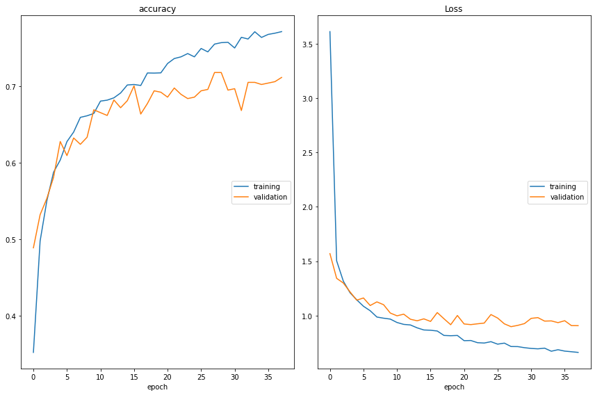
accuracy
training (min: 0.307, max: 0.628, cur: 0.628)
validation (min: 0.439, max: 0.617, cur: 0.597)
Loss
training (min: 1.070, max: 16.712, cur: 1.087)
validation (min: 1.151, max: 1.559, cur: 1.224)
99/99 [==============================] - 110s 1s/step - loss: 1.0867 - accuracy: 0.6284 - val_loss: 1.2235 - val_accuracy: 0.5965
Wall time: 52min 7s# Generate predictions
vgg_model.load_weights('tl_model_v1.weights.best.hdf5') # initialize the best trained weights
true_classes = testgen.classes
class_indices = traingen.class_indices
class_indices = dict((v,k) for k,v in class_indices.items())
vgg_preds = vgg_model.predict(testgen)
vgg_pred_classes = np.argmax(vgg_preds, axis=1)from sklearn.metrics import accuracy_score
vgg_acc = accuracy_score(true_classes, vgg_pred_classes)
print("VGG16 Model Accuracy without Fine-Tuning: {:.2f}%".format(vgg_acc * 100))VGG16 Model Accuracy without Fine-Tuning: 73.24%Using Pre-trained Layers for Fine-Tuning
Wow! What an improvement from our custom CNN! Integrating VGG16's pre-trained layers with an initialized Fully-Connected layer achieved an accuracy of 73%! But how can we do better?
In this next section, we will re-compile the model but allow for backpropagation to update the last two pre-trained layers.
You'll notice that we compile this Fine-tuning model with a lower learning rate, which will help the Fully-Connected layer "warm-up" and learn robust patterns previously learned before picking apart more minute image details.
Just as before, we'll initialize our Fully-Connected layer and its weights for training.
# Reset our image data generators
traingen.reset()
validgen.reset()
testgen.reset()
# Use a smaller learning rate
optim_2 = Adam(lr=0.0001)
# Re-compile the model, this time leaving the last 2 layers unfrozen for Fine-Tuning
vgg_model_ft = create_model(input_shape, n_classes, optim_2, fine_tune=2)%%time
plot_loss_2 = PlotLossesCallback()
# Retrain model with fine-tuning
vgg_ft_history = vgg_model_ft.fit(traingen,
batch_size=BATCH_SIZE,
epochs=n_epochs,
validation_data=validgen,
steps_per_epoch=n_steps,
validation_steps=n_val_steps,
callbacks=[tl_checkpoint_1, early_stop, plot_loss_2],
verbose=1)accuracy
training (min: 0.352, max: 0.771, cur: 0.771)
validation (min: 0.489, max: 0.718, cur: 0.711)
Loss
training (min: 0.661, max: 3.611, cur: 0.661)
validation (min: 0.898, max: 1.569, cur: 0.907)
99/99 [==============================] - 110s 1s/step - loss: 0.6611 - accuracy: 0.7712 - val_loss: 0.9069 - val_accuracy: 0.7114
Wall time: 1h 12min 19s# Generate predictions
vgg_model_ft.load_weights('tl_model_v1.weights.best.hdf5') # initialize the best trained weights
vgg_preds_ft = vgg_model_ft.predict(testgen)
vgg_pred_classes_ft = np.argmax(vgg_preds_ft, axis=1)vgg_acc_ft = accuracy_score(true_classes, vgg_pred_classes_ft)
print("VGG16 Model Accuracy with Fine-Tuning: {:.2f}%".format(vgg_acc_ft * 100))VGG16 Model Accuracy with Fine-Tuning: 81.52%An accuracy of 81%! Amazing what unfreezing the last convolutional layers can do for model performance. Let's get a better idea of how our different models have performed in classifying the data.
Comparing Models
In addition to comparing the models created in this article, we will also want to compare the last article's custom model. At the beginning of this article, we loaded the from-scratch model's learned weights, so we need to make predictions to compare against the transfer learning models.
Since our last model had a different image size target, we first need to make a new ImageDataGenerator to make predictions. Here's that code:
# Loading predictions from last article's model
test_generator = ImageDataGenerator(rescale=1/255.)
testgen = test_generator.flow_from_directory(download_dir/'food-101/test',
target_size=(128, 128),
batch_size=1,
class_mode=None,
classes=class_subset,
shuffle=False,
seed=42)
scratch_preds = scratch_model.predict(testgen)
scratch_pred_classes = np.argmax(scratch_preds, axis=1)
scratch_acc = accuracy_score(true_classes, scratch_pred_classes)
print("From Scratch Model Accuracy with Fine-Tuning: {:.2f}%".format(scratch_acc * 100))Found 2500 images belonging to 10 classes.
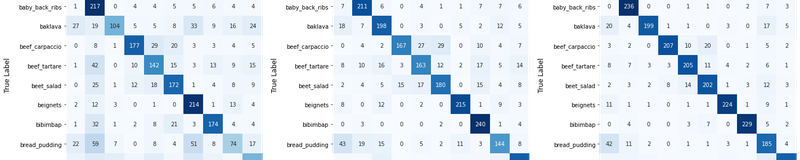
From Scratch Model Accuracy with Fine-Tuning: 56.96%We now have predictions for all three models we want to compare. Below is a function for visualizing class-wise predictions in a confusion matrix using the heatmap method Seaborn, a visualization library. Confusion matrices are NxN matrices where N is the number of classes, and predicted and target labels are plotted along the X- and Y-axes, respectively. Essentially, this tells us how many correct and incorrect classifications each model made by comparing the true class versus the predicted class. Naturally, the larger the values down the diagonal, the better the model did.
Here's our visualization code:
import seaborn as sns
from sklearn.metrics import confusion_matrix
# Get the names of the ten classes
class_names = testgen.class_indices.keys()
def plot_heatmap(y_true, y_pred, class_names, ax, title):
cm = confusion_matrix(y_true, y_pred)
sns.heatmap(
cm,
annot=True,
square=True,
xticklabels=class_names,
yticklabels=class_names,
fmt='d',
cmap=plt.cm.Blues,
cbar=False,
ax=ax
)
ax.set_title(title, fontsize=16)
ax.set_xticklabels(ax.get_xticklabels(), rotation=45, ha="right")
ax.set_ylabel('True Label', fontsize=12)
ax.set_xlabel('Predicted Label', fontsize=12)
fig, (ax1, ax2, ax3) = plt.subplots(1, 3, figsize=(20, 10))
plot_heatmap(true_classes, scratch_pred_classes, class_names, ax1, title="Custom CNN")
plot_heatmap(true_classes, vgg_pred_classes, class_names, ax2, title="Transfer Learning (VGG16) No Fine-Tuning")
plot_heatmap(true_classes, vgg_pred_classes_ft, class_names, ax3, title="Transfer Learning (VGG16) with Fine-Tuning")
fig.suptitle("Confusion Matrix Model Comparison", fontsize=24)
fig.tight_layout()
fig.subplots_adjust(top=1.25)
plt.show()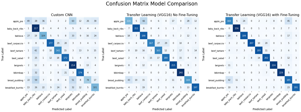
The transfer learning model with fine-tuning is the best, evident from the stronger diagonal and lighter cells everywhere else. We can also see from the confusion matrix that this model most commonly misclassifies apple pie as bread pudding. Overall, though, it's a clear winner.
Improvements
Recall that our Custom CNN accuracies, Transfer Learning Model with Feature Extraction, and Fine-Tuned Transfer Learning Model are 58%, 73%, and 81%, respectively.
We could see improved performance on our dataset as we introduce fine-tuning. Selecting the appropriate number of layers to unfreeze can require careful experimentation.
Other parameters to consider when training your network include:
- Optimizers: in this article, we used the Adam optimizer to update our weights during training. When training your network, you should experiment with other optimizers and their learning rate.
- Dropout: recall that Dropout is a form of regularization to prevent overfitting of the network. We introduced a single dropout layer in our Fully-Connected layer to constrain the network from over-learning certain features.
- Fully-Connected Layer: if you are taking a bootstrapped approach to Transfer Learning, ensure that your Fully-Connected layer is structured appropriately for the classification task. Is the number of input nodes correct for the outputted features? Do we have too many densely-connected layers?
Summary
In this article, we solved an image classification problem using a custom dataset using Transfer Learning. We saw that by employing various Transfer Learning strategies such as Fine-Tuning, we can generate a model that outperforms a custom-written CNN. Some key takeaways:
- Transfer learning can be a great starting point for training a model when you do not possess a large amount of data.
- Transfer learning requires that a model has been pre-trained on a robust source task which can be easily adapted to solve a smaller target task.
- Transfer learning is easily accessible through the Keras API. You can find available pre-trained models here.
- Fine-Tuning a portion of pre-trained layers can boost model performance significantly
Other Resources
Convolutional Neural Networks– Andrew Ng, Coursera
Andrew Ng's Deep Learning course on CNNs contains videos that offer detailed explanations of CNN concepts.
CS231n Convolutional Neural Networks for Visual Recognition– Stanford University
These notes accompany the Stanford University course and are updated regularly
Meet the Authors

James is a data science consultant and technical writer. He has spent four years working on data-driven projects and delivering machine learning solutions in the research industry.