
Ph.D. in Computer Engineering, Data Scientist
Hierarchical Clustering
LearnDataSci is reader-supported. When you purchase through links on our site, earned commissions help support our team of writers, researchers, and designers at no extra cost to you.
What is Hierarchical Clustering?
Hierarchical clustering is a popular method for grouping objects. It creates groups so that objects within a group are similar to each other and different from objects in other groups. Clusters are visually represented in a hierarchical tree called a dendrogram.
Hierarchical clustering has a couple of key benefits:
- There is no need to pre-specify the number of clusters. Instead, the dendrogram can be cut at the appropriate level to obtain the desired number of clusters.
- Data is easily summarized/organized into a hierarchy using dendrograms. Dendrograms make it easy to examine and interpret clusters.
Applications
There are many real-life applications of Hierarchical clustering. They include:
- Bioinformatics: grouping animals according to their biological features to reconstruct phylogeny trees
- Business: dividing customers into segments or forming a hierarchy of employees based on salary.
- Image processing: grouping handwritten characters in text recognition based on the similarity of the character shapes.
- Information Retrieval: categorizing search results based on the query.
Hierarchical clustering types
There are two main types of hierarchical clustering:
- Agglomerative: Initially, each object is considered to be its own cluster. According to a particular procedure, the clusters are then merged step by step until a single cluster remains. At the end of the cluster merging process, a cluster containing all the elements will be formed.
- Divisive: The Divisive method is the opposite of the Agglomerative method. Initially, all objects are considered in a single cluster. Then the division process is performed step by step until each object forms a different cluster. The cluster division or splitting procedure is carried out according to some principles that maximum distance between neighboring objects in the cluster.
Between Agglomerative and Divisive clustering, Agglomerative clustering is generally the preferred method. The below example will focus on Agglomerative clustering algorithms because they are the most popular and easiest to implement.
Hierarchical clustering steps
Hierarchical clustering employs a measure of distance/similarity to create new clusters. Steps for Agglomerative clustering can be summarized as follows:
- Step 1: Compute the proximity matrix using a particular distance metric
- Step 2: Each data point is assigned to a cluster
- Step 3: Merge the clusters based on a metric for the similarity between clusters
- Step 4: Update the distance matrix
- Step 5: Repeat Step 3 and Step 4 until only a single cluster remains
Computing a proximity matrix
The first step of the algorithm is to create a distance matrix. The values of the matrix are calculated by applying a distance function between each pair of objects. The Euclidean distance function is commonly used for this operation. The structure of the proximity matrix will be as follows for a data set with $n$ elements. Here, $d(p_i, p_j)$ represent the distance values between $p_i$ and $p_j$.
| $p_1$ | $p_2$ | $p_3$ | $...$ | $p_n$ | |
|---|---|---|---|---|---|
| $p_1$ | $d(p_1,p_1)$ | $d(p_1,p_2)$ | $d(p_1,p_3)$ | $...$ | $d(p_1,p_n)$ |
| $p_2$ | $d(p_2,p_1)$ | $d(p_2,p_2)$ | $d(p_2,p_3)$ | $...$ | $d(p_2,p_n)$ |
| $p_3$ | $d(p_3,p_1)$ | $d(p_3,p_2)$ | $d(p_3,p_3)$ | $...$ | $d(p_3,p_n)$ |
| $...$ | $...$ | $...$ | $...$ | $...$ | $...$ |
| $p_n$ | $d(p_n,p_1)$ | $d(p_n,p_2)$ | $d(p_n,p_3)$ | $...$ | $d(p_n,p_n)$ |
Similarity between Clusters
The main question in hierarchical clustering is how to calculate the distance between clusters and update the proximity matrix. There are many different approaches used to answer that question. Each approach has its advantages and disadvantages. The choice will depend on whether there is noise in the data set, whether the shape of the clusters is circular or not, and the density of the data points.
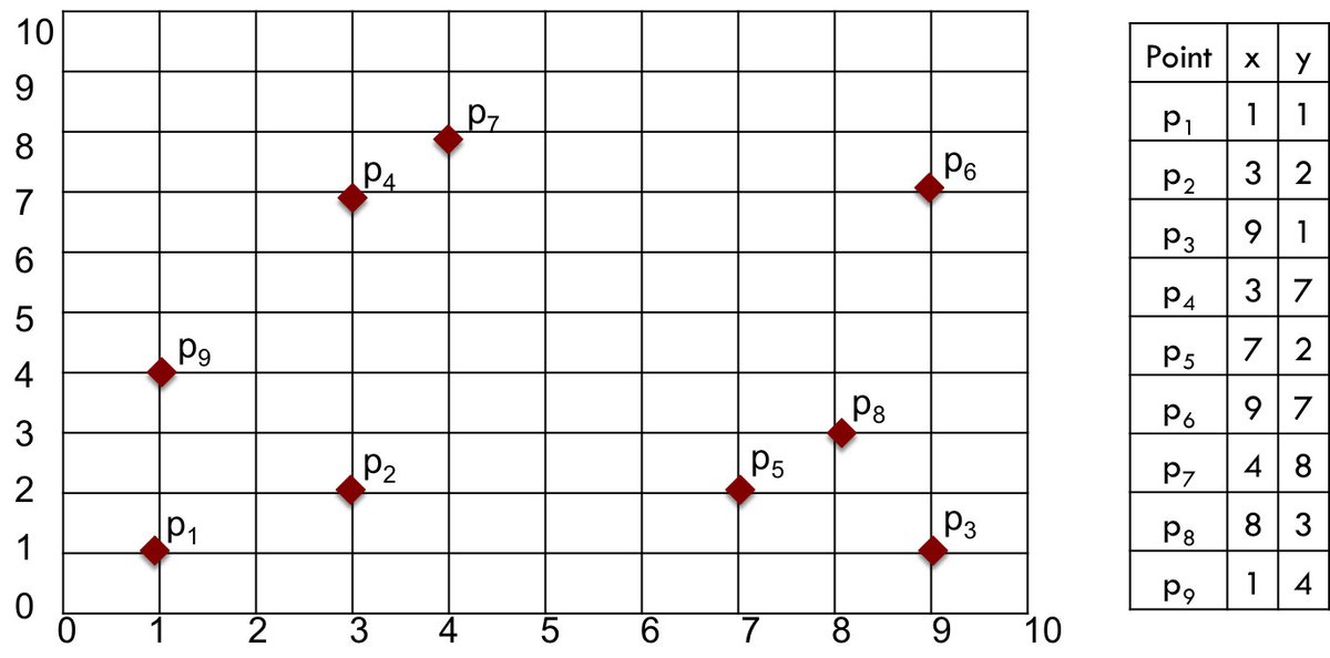
A numerical example will help illustrate the methods and choices. We'll use a small sample data set containing just nine two-dimensional points, displayed in Figure 1.
Suppose we have two clusters in the sample data set, as shown in Figure 2. There are different approaches to calculate the distance between the clusters. Popular methods are listed below.

Min (Single) Linkage
One way to measure the distance between clusters is to find the minimum distance between points in those clusters. That is, we can find the point in the first cluster nearest to a point in the other cluster and calculate the distance between those points. In Figure 2, the closest points are $p_2$ in one cluster and $p_5$ in the other. The distance between those points, and hence the distance between clusters, is found as $d(p_2, p_5) = 4$.
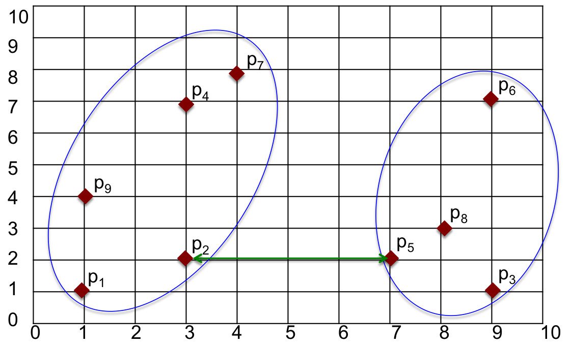
The advantage of the Min method is that it can accurately handle non-elliptical shapes. The disadvantages are that it is sensitive to noise and outliers.
Max (Complete) Linkage
Another way to measure the distance is to find the maximum distance between points in two clusters. We can find the points in each cluster that are furthest away from each other and calculate the distance between those points. In Figure 3, the maximum distance is between $p_1$ and $p_6$. Distance between those two points, and hence the distance between clusters, is found as $d(p_1, p_6) = 10$.

Max is less sensitive to noise and outliers in comparison to MIN method. However, MAX can break large clusters and tends to be biased towards globular clusters.
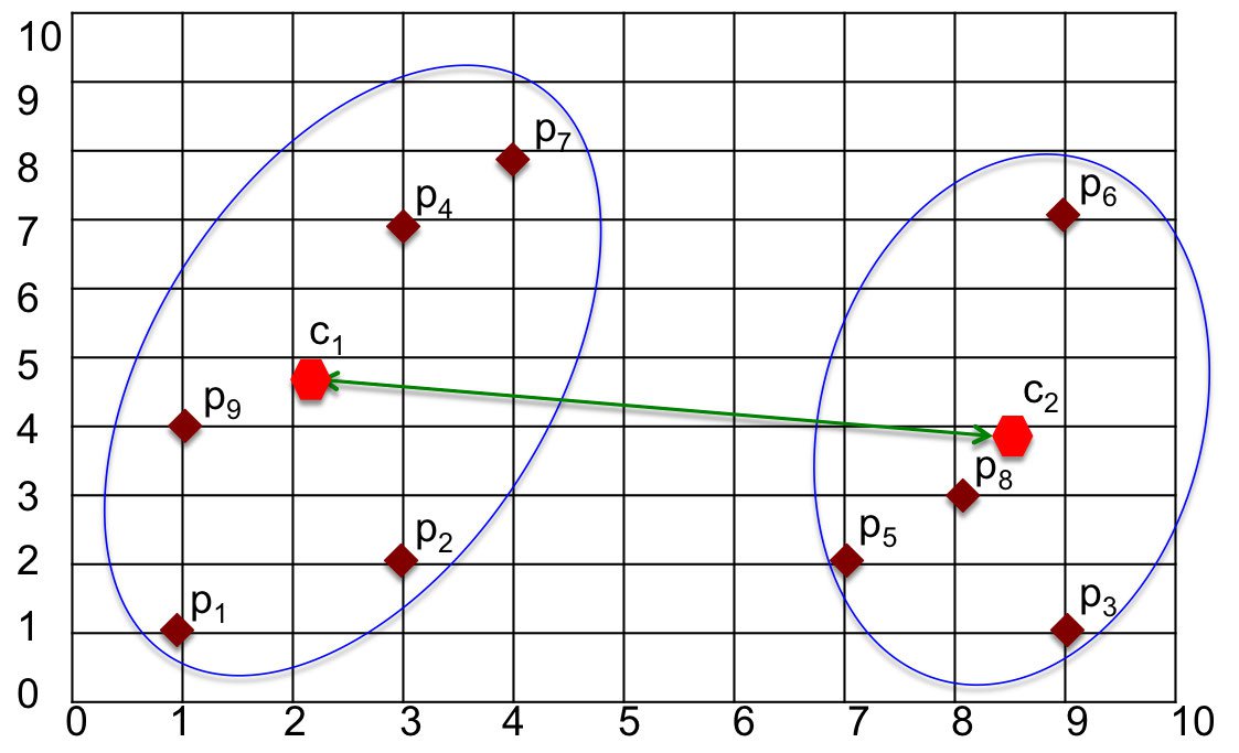
Centroid Linkage
The Centroid method defines the distance between clusters as being the distance between their centers/centroids. After calculating the centroid for each cluster, the distance between those centroids is computed using a distance function.
Average Linkage
The Average method defines the distance between clusters as the average pairwise distance among all pairs of points in the clusters. For simplicity, only some of the lines connecting pairs of points are shown in Figure 6.

Ward Linkage
The Ward approach analyzes the variance of the clusters rather than measuring distances directly, minimizing the variance between clusters.
With the Ward method, the distance between two clusters is related to how much the sum of squares (SS) value will increase when combined.
In other words, the Ward method attempts to minimize the sum of the squared distances of the points from the cluster centers. Compared to the distance-based measures described above, the Ward method is less susceptible to noise and outliers. Therefore, Ward's method is preferred more than others in clustering.
Hierarchical Clustering with Python
In Python, the Scipy and Scikit-Learn libraries have defined functions for hierarchical clustering. The below examples use these library functions to illustrate hierarchical clustering in Python.
First, we'll import NumPy, matplotlib, and seaborn (for plot styling):
import numpy as np
import matplotlib.pyplot as plt
import seaborn as sns
sns.set_style('dark')Next, we'll define a small sample data set:
X1 = np.array([[1,1], [3,2], [9,1], [3,7], [7,2], [9,7], [4,8], [8,3],[1,4]])Let's graph this data set as a scatter plot:
plt.figure(figsize=(6, 6))
plt.scatter(X1[:,0], X1[:,1], c='r')
# Create numbered labels for each point
for i in range(X1.shape[0]):
plt.annotate(str(i), xy=(X1[i,0], X1[i,1]), xytext=(3, 3), textcoords='offset points')
plt.xlabel('x coordinate')
plt.ylabel('y coordinate')
plt.title('Scatter Plot of the data')
plt.xlim([0,10]), plt.ylim([0,10])
plt.xticks(range(10)), plt.yticks(range(10))
plt.grid()
plt.show()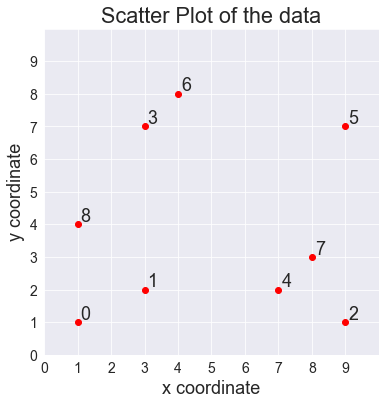
We'll now use this data set to perform hierarchical clustering.
Hierarchical Clustering using Scipy
The Scipy library has the linkage function for hierarchical (agglomerative) clustering.
The linkage function has several methods available for calculating the distance between clusters: single, average, weighted, centroid, median, and ward. We will compare these methods below. For more details on the linkage function, see the docs.
To draw the dendrogram, we'll use the dendrogram function. Again, for more details of the dendrogram function, see the docs.
First, we will import the required functions, and then we can form linkages with the various methods:
from scipy.cluster.hierarchy import dendrogram, linkage
Z1 = linkage(X1, method='single', metric='euclidean')
Z2 = linkage(X1, method='complete', metric='euclidean')
Z3 = linkage(X1, method='average', metric='euclidean')
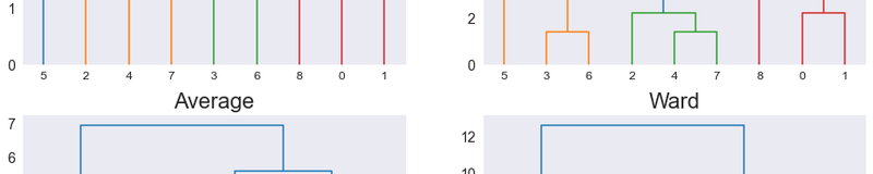
Z4 = linkage(X1, method='ward', metric='euclidean')Now, by passing the dendrogram function to matplotlib, we can view a plot of these linkages:
plt.figure(figsize=(15, 10))
plt.subplot(2,2,1), dendrogram(Z1), plt.title('Single')
plt.subplot(2,2,2), dendrogram(Z2), plt.title('Complete')
plt.subplot(2,2,3), dendrogram(Z3), plt.title('Average')
plt.subplot(2,2,4), dendrogram(Z4), plt.title('Ward')
plt.show()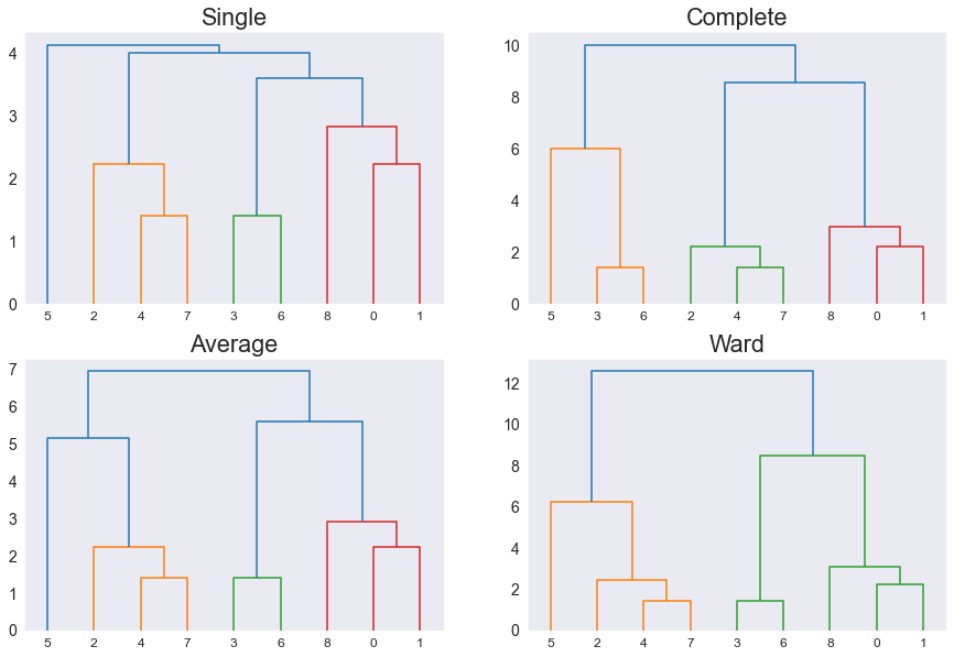
Notice that each distance method produces different linkages for the same data.
Finally, let's use the fcluster function to find the clusters for the Ward linkage:
from scipy.cluster.hierarchy import fcluster
f1 = fcluster(Z4, 2, criterion='maxclust')
print(f"Clusters: {f1}")Clusters: [2 2 1 2 1 1 2 1 2]The fcluster function gives the labels of clusters in the same index as the data set, X1. For example, index one of f1 is 2, which is the cluster for the entry at index one of X1, which is [1, 1].
X1 Cluster
[1 1] --> 2
[3 2] --> 2
[9 1] --> 1
[3 7] --> 2
[7 2] --> 1
[9 7] --> 1
[4 8] --> 2
[8 3] --> 1
[1 4] --> 2Hierarchical Clustering using Scikit-Learn
The Scikit-Learn library has its own function for agglomerative hierarchical clustering: AgglomerativeClustering.
Options for calculating the distance between clusters include ward, complete, average, and single. For more specific information, you can find this class in the relevant docs
Using sklearn is slightly different than scipy. We need to import the AgglomerativveClustering class, then instantiate it with the number of desired clusters and the distance (linkage) function to use. Then, we use fit_predict to train and predict the clusters using the X1 data set:
from sklearn.cluster import AgglomerativeClustering
Z1 = AgglomerativeClustering(n_clusters=2, linkage='ward')
Z1.fit_predict(X1)
print(Z1.labels_)[0 0 1 0 1 1 0 1 0]Again, here's a match up for each entry in X1 and its corresponding cluster:
X1 Cluster
[1 1] --> 0
[3 2] --> 0
[9 1] --> 1
[3 7] --> 0
[7 2] --> 1
[9 7] --> 1
[4 8] --> 0
[8 3] --> 1
[1 4] --> 0The following code draws a scatter plot using the cluster labels.
fig, ax = plt.subplots(figsize=(6, 6))
scatter = ax.scatter(X1[:,0], X1[:,1], c=Z1.labels_, cmap='rainbow')
legend = ax.legend(*scatter.legend_elements(), title="Clusters", bbox_to_anchor=(1, 1))
ax.add_artist(legend)
plt.title('Scatter plot of clusters')
plt.show()
Notice how the coloring of each point indicates how the data has been clustered into left and right regions.
Clustering a real dataset
In the previous section, hierarchical clustering was performed on a simple data set. In the following section, hierarchical clustering will be performed on real-world data to solve a real problem.
Here, we use a dataset from the book Biostatistics with R, which contains information for nine different protein sources and their respective consumption from various countries. We'll use this data to group countries according to their protein consumption.
First, we'll read in the CSV and display the first few rows of data:
import pandas as pd
df = pd.read_csv('https://raw.githubusercontent.com/LearnDataSci/glossary/main/data/protein.csv')
df.head()| Country | RedMeat | WhiteMeat | Eggs | Milk | Fish | Cereals | Starch | Nuts | Fr.Veg | |
|---|---|---|---|---|---|---|---|---|---|---|
| 0 | Albania | 10.1 | 1.4 | 0.5 | 8.9 | 0.2 | 42.3 | 0.6 | 5.5 | 1.7 |
| 1 | Austria | 8.9 | 14.0 | 4.3 | 19.9 | 2.1 | 28.0 | 3.6 | 1.3 | 4.3 |
| 2 | Belgium | 13.5 | 9.3 | 4.1 | 17.5 | 4.5 | 26.6 | 5.7 | 2.1 | 4.0 |
| 3 | Bulgaria | 7.8 | 6.0 | 1.6 | 8.3 | 1.2 | 56.7 | 1.1 | 3.7 | 4.2 |
| 4 | Czechoslovakia | 9.7 | 11.4 | 2.8 | 12.5 | 2.0 | 34.3 | 5.0 | 1.1 | 4.0 |
We'll first store the features for clustering in X2, which are contained in all rows and columns from 1 to 10:
X2 = df.iloc[:,1:10]Again, we use the linkage function for clustering the data:
Z2 = linkage(X2, method='ward', metric='euclidean')Finally, we can plot a dendrogram of the ward linkage clustering of 25 countries based on their protein consumption:
labelList = list(df['Country'])
plt.figure(figsize=(13, 12))
dendrogram(
Z2,
orientation='right',
labels=labelList,
distance_sort='descending',
show_leaf_counts=False,
leaf_font_size=16
)
plt.show()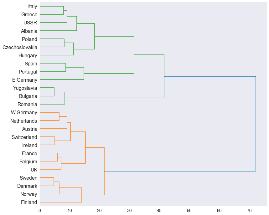
From the dendrogram, we can observe two distinct clusters colored green and yellow. This result indicates that countries in each cluster get their protein from similar sources.
Using the fcluster function, we can find and add the cluster labels for each country to the data frame.
df['Clusters'] = fcluster(Z2, 2, criterion='maxclust')
df.head()| Country | RedMeat | WhiteMeat | Eggs | Milk | Fish | Cereals | Starch | Nuts | Fr.Veg | Clusters | |
|---|---|---|---|---|---|---|---|---|---|---|---|
| 0 | Albania | 10.1 | 1.4 | 0.5 | 8.9 | 0.2 | 42.3 | 0.6 | 5.5 | 1.7 | 2 |
| 1 | Austria | 8.9 | 14.0 | 4.3 | 19.9 | 2.1 | 28.0 | 3.6 | 1.3 | 4.3 | 1 |
| 2 | Belgium | 13.5 | 9.3 | 4.1 | 17.5 | 4.5 | 26.6 | 5.7 | 2.1 | 4.0 | 1 |
| 3 | Bulgaria | 7.8 | 6.0 | 1.6 | 8.3 | 1.2 | 56.7 | 1.1 | 3.7 | 4.2 | 2 |
| 4 | Czechoslovakia | 9.7 | 11.4 | 2.8 | 12.5 | 2.0 | 34.3 | 5.0 | 1.1 | 4.0 | 2 |
From here, we can utilize this clustering result to enhance other analyses we perform on the data.
Meet the Authors

Associate Professor of Computer Engineering. Author/co-author of over 30 journal publications. Instructor of graduate/undergraduate courses. Supervisor of Graduate thesis. Consultant to IT Companies.

