
Ph.D. in Computer Engineering, Data Scientist
Eigenspace
An Eigenspace is a basic concept in linear algebra, and is commonly found in data science and in engineering and science in general.
LearnDataSci is reader-supported. When you purchase through links on our site, earned commissions help support our team of writers, researchers, and designers at no extra cost to you.
What is an Eigenspace?
For a square matrix $A$, the eigenspace of $A$ is the span of eigenvectors associated with an eigenvalue, $\lambda$.
The eigenspace can be defined mathematically as follows: $$E_{\lambda}(A) = N(A-\lambda I) $$ Where:
- $A$ is a square matrix of size $n$
- the scalar $\lambda$ is an eigenvalue associated with some eigenvector, $v$
- $N(A-\lambda I)$ is the null space of $A-\lambda I$.
If you need a refresher on eigenvalues and eigenvectors, see the video Eigenvectors and eigenvalues | Chapter 14, Essence of linear algebra, by 3Blue1Brown.
An Eigenspace is a basic concept in linear algebra, commonly found in data science and STEM in general. For example, they can be found in Principal Component Analysis (PCA), a popular dimensionality reduction technique, and in facial recognition algorithms.
A Numerical Example:
Let's consider a simple example with a matrix $A$: $$ A= \begin{bmatrix} 2 & 3 \\ 2 & 1
\end{bmatrix} $$
Step 1: Obtain eigenvalues using the characteristic polynomial given by $det(A - \lambda I)=0$.
$$ \begin{align} \det (A- \lambda I_n ) = 0 \\[5pt] \det \left( \begin{bmatrix} 2 & 3 \\ 2 & 1 \end{bmatrix} - \lambda \begin{bmatrix} 1 & 0 \\ 0 & 1 \end{bmatrix} \right) = 0 \\[5pt] \det \left( \begin{bmatrix} 2 & 3 \\ 2 & 1 \end{bmatrix} - \begin{bmatrix} \lambda & 0 \\ 0 & \lambda \end{bmatrix} \right) = 0 \\[5pt] \begin{vmatrix} 2-\lambda & 3 \\ 2 & 1-\lambda \end{vmatrix} = 0 \\[5pt] (2-\lambda)(1-\lambda) - 2 \cdot 3 = 0 \\[5pt] \lambda ^2 - 3 \lambda -4 = 0 \\[5pt] (\lambda -4)(\lambda +1) = 0 \\[5pt] \lambda_1 = 4, \ \lambda_2 = -1 \end{align} $$
The roots of the characteristic polynomial give eigenvalues $\lambda_1 = 4$ and $\lambda_2 = -1 $
Step 2: The associated eigenvectors can now be found by substituting eigenvalues $\lambda$ into $(A − \lambda I)$. Eigenvectors that correspond to these eigenvalues are calculated by looking at vectors $\vec{v}$ such that
$$ \begin{bmatrix} 2-\lambda & 3 \\ 2 & 1-\lambda \end{bmatrix} \vec{v} = 0 $$
Eigenvector for $\lambda _1 = 4 $ is found by solving the following homogeneous system of equations:
$$ \begin{bmatrix} 2-4 & 3 \\ 2 & 1-4 \end{bmatrix} \begin{bmatrix} x_1 \\ x_2 \end{bmatrix} = \begin{bmatrix} -2 & 3 \\ 2 & -3 \end{bmatrix} \begin{bmatrix} x_1 \\ x_2 \end{bmatrix} = 0 $$
After solving the above homogeneous system of equations, the first eigenvector is obtained: $$ v_1 = \begin{bmatrix} 3 \\ 2 \end{bmatrix} $$
Similarly, eigenvector for $\lambda_2 = -1$ is found.
$$ \begin{bmatrix} 2+1 & 3 \\ 2 & 1+1 \end{bmatrix} \begin{bmatrix} x_1 \\ x_2 \end{bmatrix} = \begin{bmatrix} 3 & 3 \\ 2 & 2 \end{bmatrix} \begin{bmatrix} x_1 \\ x_2 \end{bmatrix} = 0 $$
After solving the above homogeneous system of equations, the second eigenvector is obtained. $$ v_2 = \begin{bmatrix} 1 \\ -1 \end{bmatrix} $$
Step 3: After obtaining eigenvalues and eigenvectors, the eigenspace can be defined. The eigenvectors form the basis and define the eigenspace of matrix $A$ with associated eigenvalue $\lambda$. In this way, the solution space can be defined as:
$$ E_4 (A) = span(\begin{bmatrix} 3 \\ 2 \end{bmatrix}), \hspace{1cm} E_{-1}(A) = span(\begin{bmatrix} 1 \\ -1 \end{bmatrix})$$
Recall that the span of a single vector is an infinite line through the vector. Thus, $E_{4}(A)$ is the line through the origin and the point (3, 2), and $E_{−1}(A)$ is the line through the origin and the point (1, -1).
Python Example
In order to calculate eigenvectors and eigenvalues, Numpy or Scipy libraries can be used. Details of NumPy and Scipy linear algebra functions can be found from numpy.linalg and scipy.linalg , respectively. The matplotlib library will be used to plot eigenspaces.
# Import libraries
import numpy as np
import numpy.linalg as la # alternative: import scipy.linalg as la
import matplotlib.pyplot as plt
import seaborn as sns
sns.set_style("darkgrid")# Define a 2x2 square matrix
A = np.array([[2, 3],[2, 1]])
Aarray([[2, 3],
[2, 1]])Now we compute the eigenvalues and eigenvectors of the square matrix. numpy.linalg.eig computes eigenvalues and eigenvectors and returns a tuple, (eigvals, eigvecs), where eigvals is a 1D NumPy array of complex numbers giving the eigenvalues, and eigvecs is a 2D NumPy array with the corresponding eigenvectors in the columns.
eig_vals, eig_vecs = la.eig(A)
# The eigenvalues are:
lambda_1 = np.real(eig_vals[0]) # First eigenvalue
lambda_2 = np.real(eig_vals[1]) # Second eigenvalue
print('Eigenvalues: \n','lambda_1 = ', lambda_1, '\n','lambda_2 =', lambda_2, '\n')
# The corresponding eigenvectors are:
v_1 = eig_vecs[:, 0] # First eigenvector
v_2 = eig_vecs[:, 1] # Second eigenvector
print('Eigenvectors: \n', 'v_1 =', v_1,'\n', 'v_2 =', v_2)Eigenvalues:
lambda_1 = 4.0
lambda_2 = -1.0
Eigenvectors :
v_1 = [0.83205029 0.5547002 ]
v_2 = [-0.70710678 0.70710678]# Create a figure to show eigenspace
fig, ax = plt.subplots(figsize=(8, 8))
ax.grid(alpha=0.5)
ax.set(xlim=(-4, 4), ylim=(-4, 4))
ax.spines['left'].set_position('zero')
ax.spines['bottom'].set_position('zero')
sns.despine()
# Plot eigenvectors with blue arrows
for i in range(eig_vecs.shape[1]):
h1 = ax.annotate('', xy=eig_vecs[:, i], xytext=(0, 0), arrowprops={'facecolor': 'blue'})
ax.text(eig_vecs[0, i], eig_vecs[1, i] + .3, f'$v_{i}$', fontsize=16)
# Av and λv are collinear with v and the origin. Plot Av with red arrows.
for i in range(eig_vecs.shape[1]):
A_v = A @ eig_vecs[:, i] # Matrix multiplications
h2 = ax.annotate('', xy=A_v, xytext=(0, 0), arrowprops={'facecolor': 'red', 'alpha': 0.5})
ax.text(A_v[0], A_v[1] - .3, f'$Av_{i}$', fontsize=16)
# To show the eigenspace, plot the lines that run through the origin and the eigenvectors
x = np.linspace(-4, 4, 3)
for i in range(eig_vecs.shape[1]) :
a = eig_vecs[:, i][1] / eig_vecs[:, i][0] # Gradient of the eigenvectors
h3, = ax.plot(x, a * x, 'g-', lw=0.8)
ax.legend(
[h1.arrow_patch, h2.arrow_patch, h3],
('eigenvectors', r'$Av$', 'eigenspace'),
bbox_to_anchor=(1.05, 1), loc='upper left', borderaxespad=0.,
prop={'size': 15}
)
plt.show()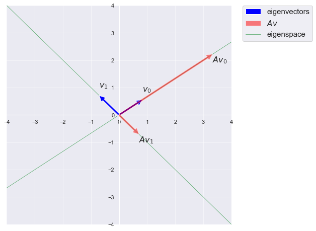
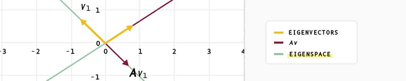
In this figure, blue arrows show the eigenvectors, red arrows represent $A\vec{v}$ which is collinear with $\vec{v}$. The eigenspaces are depicted as green lines, which are spanned by the eigenvectors.
Meet the Authors

Associate Professor of Computer Engineering. Author/co-author of over 30 journal publications. Instructor of graduate/undergraduate courses. Supervisor of Graduate thesis. Consultant to IT Companies.