
Ph.D. in Computer Engineering, Data Scientist
Chebyshev's Inequality
LearnDataSci is reader-supported. When you purchase through links on our site, earned commissions help support our team of writers, researchers, and designers at no extra cost to you.
What is Chebyshev's Inequality
Chebyshev's inequality is a theory describing the maximum number of extreme values in a probability distribution. It states that no more than a certain percentage of values ($1/k^2$) will be beyond a given distance ($k$ standard deviations) from the distribution’s average. The theorem is particularly useful because it can be applied to any probability distribution, even ones that violate normality, so long as the mean and variance are known. The equation is:
$$ Pr(|X-\mu| \geq k \times \sigma) \leq \frac{1}{k^2} $$
In plain English, the formula says that the probability of a value (X) being more than k standard deviations (𝜎) away from the mean (𝜇) is less than or equal to $1/k^2$. In that formula, $k$ represents a distance away from the mean expressed in standard deviation units, where $k$ can take any above-zero value.
As an example, let's calculate the probability for $k=2$.
$$ Pr(|X-\mu | \geq k) \leq \frac{\sigma^2}{k^2} $$
Although, the inequality is valid for any real number $k>0$, only the case $k>1$ is practically useful.
As an example, let's calculate the probability for k=2.
$$ Pr(|X-\mu|\geq 2 \times \sigma) \leq \frac{1}{4} $$
The answer is that no more than ¼ of values will be more than 2 standard deviations away from the distribution’s mean. Note that this is a loose upper bound, but it is valid for any distribution.
Finding the reverse: Number of values within a range
Chebyshev’s inequality can also be used to find the reverse information. Knowing the percentage of values outside a given range also by definition communicates the percentage of values inside that range. $\text{Percentage inside} = 1 - \text{Percentage outside}$. In other words, the maximum number of values within $k$ standard deviations of the mean will be $1 – 1/k^2$.
In the previous example, we calculated that no more $1/4$ of values will be more than 2 standard deviations away from the distribution’s mean. To find the reverse, we calculate $1 - 1/k^2 = 1 - 1/4 = 3/4$. In other words, no more than $3/4$ of values will be within 2 standard deviations from the distribution’s mean.
Applications
Chebyshev's inequality theorem is one of many (e.g., Markov’s inequality theorem) helping to describe the characteristics of probability distributions. The theorems are useful in detecting outliers and in clustering data into groups.
A Numerical Example
Suppose a fair coin is tossed 50 times. The bound on the probability that the number of heads will be greater than 35 or less than 15 can be found using Chebyshev's Inequality.
Let $X$ be the number of heads. Because $X$ has a binomial distribution:
- The expected value will be: $ \mu = n \times p = 50 \times 0.5 = 25$
- The variance will be: $ \sigma^2 = n \times p \times (1-p) = 50 \times 0.5 \times 0.5 = 12.5 $
- The standard deviation will be $\sqrt{\sigma^2} = \sqrt{12.5}$
- The value 35 and 15 are 10 away from the average, which is 2.8284 standard deviations (ie, $10 / \sqrt{12.5}$)
Using Chebyshev's Inequality we can write the following probability:
$$Pr( X <15 \cup X>35) = Pr(|X - \mu| \geq k \times \sigma) \leq \frac{1}{k^2} = \frac{1}{2.8284^2} = 0.125$$
In other words, chances of a fair coin coming up heads outside the range of 15 to 35 times is at most 0.125.
Python Implementation
We'll first import a few libraries that will help us work with Chebyshev:
import numpy as np
import matplotlib.pyplot as plt
from scipy.stats import normChebyshev's inequality can be written as a simple function:
def chebyshev_inequality(k):
return 1 / k**2We'll now use this function to find probability for different k values. First, we'll create an array of 10 numbers that have a distance of 0.5 between values. Let’s also initialize an array of zeros of the same length in order to hold the probability results we’re about to calculate.
k = np.arange(1,10,0.5)
p_cheb = np.zeros(len(k))
print('Chebyshev_Inequality for different k values:\n')
for i in range(len(k)):
p_cheb[i] = chebyshev_inequality(k[i])
print(f'Pr( |𝜇−𝜎| >= {k[i]}𝜎 ) <= {p_cheb[i]}' )Chebyshev_Inequality for different k values:
Pr( |𝜇−𝜎| >= 1.0𝜎 ) <= 1.0
Pr( |𝜇−𝜎| >= 1.5𝜎 ) <= 0.4444444444444444
Pr( |𝜇−𝜎| >= 2.0𝜎 ) <= 0.25
Pr( |𝜇−𝜎| >= 2.5𝜎 ) <= 0.16
Pr( |𝜇−𝜎| >= 3.0𝜎 ) <= 0.1111111111111111
Pr( |𝜇−𝜎| >= 3.5𝜎 ) <= 0.08163265306122448
Pr( |𝜇−𝜎| >= 4.0𝜎 ) <= 0.0625
Pr( |𝜇−𝜎| >= 4.5𝜎 ) <= 0.04938271604938271
Pr( |𝜇−𝜎| >= 5.0𝜎 ) <= 0.04
Pr( |𝜇−𝜎| >= 5.5𝜎 ) <= 0.03305785123966942
Pr( |𝜇−𝜎| >= 6.0𝜎 ) <= 0.027777777777777776
Pr( |𝜇−𝜎| >= 6.5𝜎 ) <= 0.023668639053254437
Pr( |𝜇−𝜎| >= 7.0𝜎 ) <= 0.02040816326530612
Pr( |𝜇−𝜎| >= 7.5𝜎 ) <= 0.017777777777777778
Pr( |𝜇−𝜎| >= 8.0𝜎 ) <= 0.015625
Pr( |𝜇−𝜎| >= 8.5𝜎 ) <= 0.01384083044982699
Pr( |𝜇−𝜎| >= 9.0𝜎 ) <= 0.012345679012345678
Pr( |𝜇−𝜎| >= 9.5𝜎 ) <= 0.0110803324099723For comparison, find the probability for unit normal distiribution, which we'll plot in the next step:
p_norm = np.zeros(len(k))
for i in range(len(k)):
p_norm[i] = (1 - norm.cdf(k[i])) * 2Now, we'll plot the probability for Normal Distribution and Chebyshev Inequality:
plt.plot(k,p_cheb, '-o')
plt.plot(k,p_norm, '-o')
plt.xlabel('k parameter')
plt.ylabel('Probability')
plt.legend(["Estimated by Chebyshev's Inequality","Estimated by Cumulative Normal Distribution"]);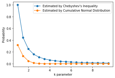
The figure shows that Chebyshev's Inequality provides an upper bound (the blue curve) for the true ratio of large numbers that can be drawn from a unit normal distribution (the orange curve). Note that Chebyshevs's Inequality provides tighter bounds for larger k values.
A Python Example
We will load the penguins dataset from the seaborn library to observe Chebyshev's Inequality. In the dataset, the flipper_length_mm variable will be used to estimate an interval using the k parameter.
First, we'll plot the distribution of flipper length:
import seaborn as sns
penguins = sns.load_dataset("penguins")
sns.displot(penguins, x="flipper_length_mm", kde=True);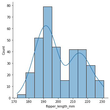
The figure shows that the the variable does not follow a normal curve. Nonetheless, we can still use Chesbyshev's Inequality for estimation.
Let's now calculate the mean and standard deviation for our calculations:
mu_flipper_lenth = penguins["flipper_length_mm"].mean()
std_flipper_lenth = penguins["flipper_length_mm"].std()
print(f"Mean of the variable is {mu_flipper_lenth}")
print(f"Standard Deviation of the variable is {std_flipper_lenth}")Mean of the variable is 200.91520467836258
Standard Deviation of the variable is 14.061713679356888Using the mean, standard deviation, and the k parameter, we can now find the upper and lower bound:
k = 2
upper_bound = mu_flipper_lenth + k * std_flipper_lenth
lower_bound = mu_flipper_lenth - k * std_flipper_lenth
print(f"Upper bound for k={k} is {upper_bound}")
print(f"Lower bound for k={k} is {lower_bound}")Upper bound for k=2 is 229.03863203707635
Lower bound for k=2 is 172.79177731964882We can obtain a kernel density function using the KernelDensity class from the sklearn library:
from sklearn.neighbors import KernelDensity
# Drop NaN values in the variable
X = penguins["flipper_length_mm"].dropna()
# Convert to numpy ndarray
X = np.array(X).reshape((len(X), 1))
# Fit a Kernel Density Model
kde = KernelDensity(bandwidth=3).fit(X)
# Estimate new variables using kde model
new_X = np.linspace(np.min(X), np.max(X), 1000)[:, np.newaxis]
log_dens = kde.score_samples(new_X)Now, let's plot the density model:
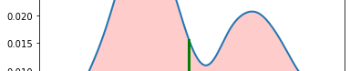
plt.plot(new_X,np.exp(log_dens), lw=2)
# Draw a vertical line to show mean
line_mu_y = np.exp(kde.score_samples(np.array(mu_flipper_lenth, dtype=object).reshape(1,1)))
plt.plot([mu_flipper_lenth, mu_flipper_lenth], [0, line_mu_y[0]], c='g', lw=3)
# Draw a vertical line for upper bound
line_upper_y = np.exp(kde.score_samples(np.array(upper_bound).reshape(1,1)))
plt.plot([upper_bound, upper_bound], [0, line_upper_y[0]], c='r', lw=3)
# Draw a vertical line for lower bound
line_lower_y = np.exp(kde.score_samples(np.array(lower_bound).reshape(1,1)))
plt.plot([lower_bound, lower_bound], [0, line_lower_y[0]], c='r', lw=3)
# Fill under the curve between upper bound and lower bound.
ptx = np.linspace(lower_bound, upper_bound, 100)
pty = np.exp(kde.score_samples(ptx.reshape(len(ptx),1)))
plt.fill_between(ptx, pty, color='r', alpha=0.2)
plt.ylim(0, )
plt.show()
Here, the red lines indicate lower-bound and upper-bound for k=2. The green vertical line shows the mean of the data. The filled area under the curve shows the values between $\mu-2\sigma$ and $\mu-2\sigma$.
Using the results, we can easily detect outliers. The values higher than upper-bound and the values less than lower-bound can be flagged as outliers.
Here's how to find the values less than lower_bound:
penguins["flipper_length_mm"][penguins["flipper_length_mm"] < lower_bound]28 172.0
Name: flipper_length_mm, dtype: float64And the values higher than upper_bound:
penguins["flipper_length_mm"][penguins["flipper_length_mm"] > upper_bound]221 230.0
253 230.0
283 231.0
285 230.0
295 230.0
309 230.0
333 230.0
335 230.0
Name: flipper_length_mm, dtype: float64Meet the Authors

Associate Professor of Computer Engineering. Author/co-author of over 30 journal publications. Instructor of graduate/undergraduate courses. Supervisor of Graduate thesis. Consultant to IT Companies.