

Data Scientist

Founder of LearnDataSci

Lead Data Scientist & ML Developer
Python Pandas Tutorial: A Complete Introduction for Beginners
Learn some of the most important pandas features for exploring, cleaning, transforming, visualizing, and learning from data.
LearnDataSci is reader-supported. When you purchase through links on our site, earned commissions help support our team of writers, researchers, and designers at no extra cost to you.
You should already know:
- Python fundamentals – you should have beginner to intermediate-level knowledge, which can be learned from most entry-level Python courses
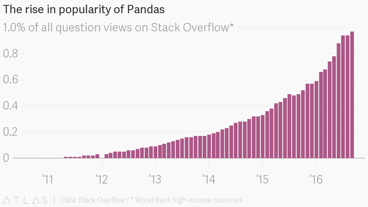
The pandas package is the most important tool at the disposal of Data Scientists and Analysts working in Python today. The powerful machine learning and glamorous visualization tools may get all the attention, but pandas is the backbone of most data projects.
[pandas] is derived from the term "panel data", an econometrics term for data sets that include observations over multiple time periods for the same individuals. — Wikipedia
If you're thinking about data science as a career, then it is imperative that one of the first things you do is learn pandas. In this post, we will go over the essential bits of information about pandas, including how to install it, its uses, and how it works with other common Python data analysis packages such as matplotlib and scikit-learn.
Article Resources
- iPython notebook and data available on GitHub
Other articles in this series
What's Pandas for?
Pandas has so many uses that it might make sense to list the things it can't do instead of what it can do.
This tool is essentially your data’s home. Through pandas, you get acquainted with your data by cleaning, transforming, and analyzing it.
For example, say you want to explore a dataset stored in a CSV on your computer. Pandas will extract the data from that CSV into a DataFrame — a table, basically — then let you do things like:
- Calculate statistics and answer questions about the data, like
- What's the average, median, max, or min of each column?
- Does column A correlate with column B?
- What does the distribution of data in column C look like?
- Clean the data by doing things like removing missing values and filtering rows or columns by some criteria
- Visualize the data with help from Matplotlib. Plot bars, lines, histograms, bubbles, and more.
- Store the cleaned, transformed data back into a CSV, other file or database
Before you jump into the modeling or the complex visualizations you need to have a good understanding of the nature of your dataset and pandas is the best avenue through which to do that.
How does pandas fit into the data science toolkit?
Not only is the pandas library a central component of the data science toolkit but it is used in conjunction with other libraries in that collection.
Pandas is built on top of the NumPy package, meaning a lot of the structure of NumPy is used or replicated in Pandas. Data in pandas is often used to feed statistical analysis in SciPy, plotting functions from Matplotlib, and machine learning algorithms in Scikit-learn.
Jupyter Notebooks offer a good environment for using pandas to do data exploration and modeling, but pandas can also be used in text editors just as easily.
Jupyter Notebooks give us the ability to execute code in a particular cell as opposed to running the entire file. This saves a lot of time when working with large datasets and complex transformations. Notebooks also provide an easy way to visualize pandas’ DataFrames and plots. As a matter of fact, this article was created entirely in a Jupyter Notebook.
When should you start using pandas?
If you do not have any experience coding in Python, then you should stay away from learning pandas until you do. You don’t have to be at the level of the software engineer, but you should be adept at the basics, such as lists, tuples, dictionaries, functions, and iterations. Also, I’d also recommend familiarizing yourself with NumPy due to the similarities mentioned above.
If you're looking for a good place to learn Python, Python for Everybody on Coursera is great (and Free).
Moreover, for those of you looking to do a data science bootcamp or some other accelerated data science education program, it's highly recommended you start learning pandas on your own before you start the program.
Even though accelerated programs teach you pandas, better skills beforehand means you'll be able to maximize time for learning and mastering the more complicated material.
Pandas First Steps
Install and import
Pandas is an easy package to install. Open up your terminal program (for Mac users) or command line (for PC users) and install it using either of the following commands:
conda install pandas
OR
pip install pandas
Alternatively, if you're currently viewing this article in a Jupyter notebook you can run this cell:
!pip install pandasThe ! at the beginning runs cells as if they were in a terminal.
To import pandas we usually import it with a shorter name since it's used so much:
import pandas as pdNow to the basic components of pandas.
Core components of pandas: Series and DataFrames
The primary two components of pandas are the Series and DataFrame.
A Series is essentially a column, and a DataFrame is a multi-dimensional table made up of a collection of Series.
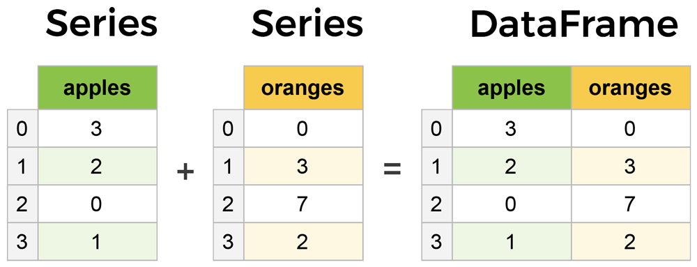
DataFrames and Series are quite similar in that many operations that you can do with one you can do with the other, such as filling in null values and calculating the mean.
You'll see how these components work when we start working with data below.
Creating DataFrames from scratch
Creating DataFrames right in Python is good to know and quite useful when testing new methods and functions you find in the pandas docs.
There are many ways to create a DataFrame from scratch, but a great option is to just use a simple dict.
Let's say we have a fruit stand that sells apples and oranges. We want to have a column for each fruit and a row for each customer purchase. To organize this as a dictionary for pandas we could do something like:
data = {
'apples': [3, 2, 0, 1],
'oranges': [0, 3, 7, 2]
}And then pass it to the pandas DataFrame constructor:
purchases = pd.DataFrame(data)
purchases| apples | oranges | |
|---|---|---|
| 0 | 3 | 0 |
| 1 | 2 | 3 |
| 2 | 0 | 7 |
| 3 | 1 | 2 |
How did that work?
Each (key, value) item in data corresponds to a column in the resulting DataFrame.
The Index of this DataFrame was given to us on creation as the numbers 0-3, but we could also create our own when we initialize the DataFrame.
Let's have customer names as our index:
purchases = pd.DataFrame(data, index=['June', 'Robert', 'Lily', 'David'])
purchases| apples | oranges | |
|---|---|---|
| June | 3 | 0 |
| Robert | 2 | 3 |
| Lily | 0 | 7 |
| David | 1 | 2 |
So now we could locate a customer's order by using their name:
purchases.loc['June']apples 3
oranges 0
Name: June, dtype: int64There's more on locating and extracting data from the DataFrame later, but now you should be able to create a DataFrame with any random data to learn on.
Let's move on to some quick methods for creating DataFrames from various other sources.
How to read in data
It’s quite simple to load data from various file formats into a DataFrame. In the following examples we'll keep using our apples and oranges data, but this time it's coming from various files.
Reading data from CSVs
With CSV files all you need is a single line to load in the data:
df = pd.read_csv('purchases.csv')
df| Unnamed: 0 | apples | oranges | |
|---|---|---|---|
| 0 | June | 3 | 0 |
| 1 | Robert | 2 | 3 |
| 2 | Lily | 0 | 7 |
| 3 | David | 1 | 2 |
CSVs don't have indexes like our DataFrames, so all we need to do is just designate the index_col when reading:
df = pd.read_csv('purchases.csv', index_col=0)
df| apples | oranges | |
|---|---|---|
| June | 3 | 0 |
| Robert | 2 | 3 |
| Lily | 0 | 7 |
| David | 1 | 2 |
Here we're setting the index to be column zero.
You'll find that most CSVs won't ever have an index column and so usually you don't have to worry about this step.
Reading data from JSON
If you have a JSON file — which is essentially a stored Python dict — pandas can read this just as easily:
df = pd.read_json('purchases.json')
df| apples | oranges | |
|---|---|---|
| David | 1 | 2 |
| June | 3 | 0 |
| Lily | 0 | 7 |
| Robert | 2 | 3 |
Notice this time our index came with us correctly since using JSON allowed indexes to work through nesting. Feel free to open data_file.json in a notepad so you can see how it works.
Pandas will try to figure out how to create a DataFrame by analyzing structure of your JSON, and sometimes it doesn't get it right. Often you'll need to set the orient keyword argument depending on the structure, so check out read_json docs about that argument to see which orientation you're using.
Reading data from a SQL database
If you’re working with data from a SQL database you need to first establish a connection using an appropriate Python library, then pass a query to pandas. Here we'll use SQLite to demonstrate.
First, we need pysqlite3 installed, so run this command in your terminal:
pip install pysqlite3
Or run this cell if you're in a notebook:
!pip install pysqlite3sqlite3 is used to create a connection to a database which we can then use to generate a DataFrame through a SELECT query.
So first we'll make a connection to a SQLite database file:
import sqlite3
con = sqlite3.connect("database.db")SQL Tip
If you have data in PostgreSQL, MySQL, or some other SQL server, you'll need to obtain the right Python library to make a connection. For example, psycopg2 (link) is a commonly used library for making connections to PostgreSQL. Furthermore, you would make a connection to a database URI instead of a file like we did here with SQLite.
For a great course on SQL check out The Complete SQL Bootcamp on Udemy
In this SQLite database we have a table called purchases, and our index is in a column called "index".
By passing a SELECT query and our con, we can read from the purchases table:
df = pd.read_sql_query("SELECT * FROM purchases", con)
df| index | apples | oranges | |
|---|---|---|---|
| 0 | June | 3 | 0 |
| 1 | Robert | 2 | 3 |
| 2 | Lily | 0 | 7 |
| 3 | David | 1 | 2 |
Just like with CSVs, we could pass index_col='index', but we can also set an index after-the-fact:
df = df.set_index('index')
df| apples | oranges | |
|---|---|---|
| index | ||
| June | 3 | 0 |
| Robert | 2 | 3 |
| Lily | 0 | 7 |
| David | 1 | 2 |
In fact, we could use set_index() on any DataFrame using any column at any time. Indexing Series and DataFrames is a very common task, and the different ways of doing it is worth remembering.
Converting back to a CSV, JSON, or SQL
So after extensive work on cleaning your data, you’re now ready to save it as a file of your choice. Similar to the ways we read in data, pandas provides intuitive commands to save it:
df.to_csv('new_purchases.csv')
df.to_json('new_purchases.json')
df.to_sql('new_purchases', con)When we save JSON and CSV files, all we have to input into those functions is our desired filename with the appropriate file extension. With SQL, we’re not creating a new file but instead inserting a new table into the database using our con variable from before.
Let's move on to importing some real-world data and detailing a few of the operations you'll be using a lot.
Most important DataFrame operations
DataFrames possess hundreds of methods and other operations that are crucial to any analysis. As a beginner, you should know the operations that perform simple transformations of your data and those that provide fundamental statistical analysis.
Let's load in the IMDB movies dataset to begin:
movies_df = pd.read_csv("IMDB-Movie-Data.csv", index_col="Title")We're loading this dataset from a CSV and designating the movie titles to be our index.
Viewing your data
The first thing to do when opening a new dataset is print out a few rows to keep as a visual reference. We accomplish this with .head():
movies_df.head()| Rank | Genre | Description | Director | Actors | Year | Runtime (Minutes) | Rating | Votes | Revenue (Millions) | Metascore | |
|---|---|---|---|---|---|---|---|---|---|---|---|
| Title | |||||||||||
| Guardians of the Galaxy | 1 | Action,Adventure,Sci-Fi | A group of intergalactic criminals are forced ... | James Gunn | Chris Pratt, Vin Diesel, Bradley Cooper, Zoe S... | 2014 | 121 | 8.1 | 757074 | 333.13 | 76.0 |
| Prometheus | 2 | Adventure,Mystery,Sci-Fi | Following clues to the origin of mankind, a te... | Ridley Scott | Noomi Rapace, Logan Marshall-Green, Michael Fa... | 2012 | 124 | 7.0 | 485820 | 126.46 | 65.0 |
| Split | 3 | Horror,Thriller | Three girls are kidnapped by a man with a diag... | M. Night Shyamalan | James McAvoy, Anya Taylor-Joy, Haley Lu Richar... | 2016 | 117 | 7.3 | 157606 | 138.12 | 62.0 |
| Sing | 4 | Animation,Comedy,Family | In a city of humanoid animals, a hustling thea... | Christophe Lourdelet | Matthew McConaughey,Reese Witherspoon, Seth Ma... | 2016 | 108 | 7.2 | 60545 | 270.32 | 59.0 |
| Suicide Squad | 5 | Action,Adventure,Fantasy | A secret government agency recruits some of th... | David Ayer | Will Smith, Jared Leto, Margot Robbie, Viola D... | 2016 | 123 | 6.2 | 393727 | 325.02 | 40.0 |
.head() outputs the first five rows of your DataFrame by default, but we could also pass a number as well: movies_df.head(10) would output the top ten rows, for example.
To see the last five rows use .tail(). tail() also accepts a number, and in this case we printing the bottom two rows.:
movies_df.tail(2)| Rank | Genre | Description | Director | Actors | Year | Runtime (Minutes) | Rating | Votes | Revenue (Millions) | Metascore | |
|---|---|---|---|---|---|---|---|---|---|---|---|
| Title | |||||||||||
| Search Party | 999 | Adventure,Comedy | A pair of friends embark on a mission to reuni... | Scot Armstrong | Adam Pally, T.J. Miller, Thomas Middleditch,Sh... | 2014 | 93 | 5.6 | 4881 | NaN | 22.0 |
| Nine Lives | 1000 | Comedy,Family,Fantasy | A stuffy businessman finds himself trapped ins... | Barry Sonnenfeld | Kevin Spacey, Jennifer Garner, Robbie Amell,Ch... | 2016 | 87 | 5.3 | 12435 | 19.64 | 11.0 |
Typically when we load in a dataset, we like to view the first five or so rows to see what's under the hood. Here we can see the names of each column, the index, and examples of values in each row.
You'll notice that the index in our DataFrame is the Title column, which you can tell by how the word Title is slightly lower than the rest of the columns.
Getting info about your data
.info() should be one of the very first commands you run after loading your data:
movies_df.info()<class 'pandas.core.frame.DataFrame'>
Index: 1000 entries, Guardians of the Galaxy to Nine Lives
Data columns (total 11 columns):
Rank 1000 non-null int64
Genre 1000 non-null object
Description 1000 non-null object
Director 1000 non-null object
Actors 1000 non-null object
Year 1000 non-null int64
Runtime (Minutes) 1000 non-null int64
Rating 1000 non-null float64
Votes 1000 non-null int64
Revenue (Millions) 872 non-null float64
Metascore 936 non-null float64
dtypes: float64(3), int64(4), object(4)
memory usage: 93.8+ KB.info() provides the essential details about your dataset, such as the number of rows and columns, the number of non-null values, what type of data is in each column, and how much memory your DataFrame is using.
Notice in our movies dataset we have some obvious missing values in the Revenue and Metascore columns. We'll look at how to handle those in a bit.
Seeing the datatype quickly is actually quite useful. Imagine you just imported some JSON and the integers were recorded as strings. You go to do some arithmetic and find an "unsupported operand" Exception because you can't do math with strings. Calling .info() will quickly point out that your column you thought was all integers are actually string objects.
Another fast and useful attribute is .shape, which outputs just a tuple of (rows, columns):
movies_df.shape(1000, 11)Note that .shape has no parentheses and is a simple tuple of format (rows, columns). So we have 1000 rows and 11 columns in our movies DataFrame.
You'll be going to .shape a lot when cleaning and transforming data. For example, you might filter some rows based on some criteria and then want to know quickly how many rows were removed.
Handling duplicates
This dataset does not have duplicate rows, but it is always important to verify you aren't aggregating duplicate rows.
To demonstrate, let's simply just double up our movies DataFrame by appending it to itself:
temp_df = movies_df.append(movies_df)
temp_df.shape(2000, 11)Using append() will return a copy without affecting the original DataFrame. We are capturing this copy in temp so we aren't working with the real data.
Notice call .shape quickly proves our DataFrame rows have doubled.
Now we can try dropping duplicates:
temp_df = temp_df.drop_duplicates()
temp_df.shape(1000, 11)Just like append(), the drop_duplicates() method will also return a copy of your DataFrame, but this time with duplicates removed. Calling .shape confirms we're back to the 1000 rows of our original dataset.
It's a little verbose to keep assigning DataFrames to the same variable like in this example. For this reason, pandas has the inplace keyword argument on many of its methods. Using inplace=True will modify the DataFrame object in place:
temp_df.drop_duplicates(inplace=True)Now our temp_df will have the transformed data automatically.
Another important argument for drop_duplicates() is keep, which has three possible options:
first: (default) Drop duplicates except for the first occurrence.last: Drop duplicates except for the last occurrence.False: Drop all duplicates.
Since we didn't define the keep arugment in the previous example it was defaulted to first. This means that if two rows are the same pandas will drop the second row and keep the first row. Using last has the opposite effect: the first row is dropped.
keep, on the other hand, will drop all duplicates. If two rows are the same then both will be dropped. Watch what happens to temp_df:
temp_df = movies_df.append(movies_df) # make a new copy
temp_df.drop_duplicates(inplace=True, keep=False)
temp_df.shape(0, 11)Since all rows were duplicates, keep=False dropped them all resulting in zero rows being left over. If you're wondering why you would want to do this, one reason is that it allows you to locate all duplicates in your dataset. When conditional selections are shown below you'll see how to do that.
Column cleanup
Many times datasets will have verbose column names with symbols, upper and lowercase words, spaces, and typos. To make selecting data by column name easier we can spend a little time cleaning up their names.
Here's how to print the column names of our dataset:
movies_df.columnsIndex(['Rank', 'Genre', 'Description', 'Director', 'Actors', 'Year',
'Runtime (Minutes)', 'Rating', 'Votes', 'Revenue (Millions)',
'Metascore'],
dtype='object')Not only does .columns come in handy if you want to rename columns by allowing for simple copy and paste, it's also useful if you need to understand why you are receiving a Key Error when selecting data by column.
We can use the .rename() method to rename certain or all columns via a dict. We don't want parentheses, so let's rename those:
movies_df.rename(columns={
'Runtime (Minutes)': 'Runtime',
'Revenue (Millions)': 'Revenue_millions'
}, inplace=True)
movies_df.columnsIndex(['Rank', 'Genre', 'Description', 'Director', 'Actors', 'Year', 'Runtime',
'Rating', 'Votes', 'Revenue_millions', 'Metascore'],
dtype='object')Excellent. But what if we want to lowercase all names? Instead of using .rename() we could also set a list of names to the columns like so:
movies_df.columns = ['rank', 'genre', 'description', 'director', 'actors', 'year', 'runtime',
'rating', 'votes', 'revenue_millions', 'metascore']
movies_df.columnsIndex(['rank', 'genre', 'description', 'director', 'actors', 'year', 'runtime',
'rating', 'votes', 'revenue_millions', 'metascore'],
dtype='object')But that's too much work. Instead of just renaming each column manually we can do a list comprehension:
movies_df.columns = [col.lower() for col in movies_df]
movies_df.columnsIndex(['rank', 'genre', 'description', 'director', 'actors', 'year', 'runtime',
'rating', 'votes', 'revenue_millions', 'metascore'],
dtype='object')list (and dict) comprehensions come in handy a lot when working with pandas and data in general.
It's a good idea to lowercase, remove special characters, and replace spaces with underscores if you'll be working with a dataset for some time.
How to work with missing values
When exploring data, you’ll most likely encounter missing or null values, which are essentially placeholders for non-existent values. Most commonly you'll see Python's None or NumPy's np.nan, each of which are handled differently in some situations.
There are two options in dealing with nulls:
- Get rid of rows or columns with nulls
- Replace nulls with non-null values, a technique known as imputation
Let's calculate to total number of nulls in each column of our dataset. The first step is to check which cells in our DataFrame are null:
movies_df.isnull()| rank | genre | description | director | actors | year | runtime | rating | votes | revenue_millions | metascore | |
|---|---|---|---|---|---|---|---|---|---|---|---|
| Title | |||||||||||
| Guardians of the Galaxy | False | False | False | False | False | False | False | False | False | False | False |
| Prometheus | False | False | False | False | False | False | False | False | False | False | False |
| Split | False | False | False | False | False | False | False | False | False | False | False |
| Sing | False | False | False | False | False | False | False | False | False | False | False |
| Suicide Squad | False | False | False | False | False | False | False | False | False | False | False |
Notice isnull() returns a DataFrame where each cell is either True or False depending on that cell's null status.
To count the number of nulls in each column we use an aggregate function for summing:
movies_df.isnull().sum()rank 0
genre 0
description 0
director 0
actors 0
year 0
runtime 0
rating 0
votes 0
revenue_millions 128
metascore 64
dtype: int64.isnull() just by iteself isn't very useful, and is usually used in conjunction with other methods, like sum().
We can see now that our data has 128 missing values for revenue_millions and 64 missing values for metascore.
Removing null values
Data Scientists and Analysts regularly face the dilemma of dropping or imputing null values, and is a decision that requires intimate knowledge of your data and its context. Overall, removing null data is only suggested if you have a small amount of missing data.
Remove nulls is pretty simple:
movies_df.dropna()This operation will delete any row with at least a single null value, but it will return a new DataFrame without altering the original one. You could specify inplace=True in this method as well.
So in the case of our dataset, this operation would remove 128 rows where revenue_millions is null and 64 rows where metascore is null. This obviously seems like a waste since there's perfectly good data in the other columns of those dropped rows. That's why we'll look at imputation next.
Other than just dropping rows, you can also drop columns with null values by setting axis=1:
movies_df.dropna(axis=1)In our dataset, this operation would drop the revenue_millions and metascore columns
Intuition
What's with this axis=1parameter?
It's not immediately obvious where axis comes from and why you need it to be 1 for it to affect columns. To see why, just look at the .shape output:
movies_df.shape
Out: (1000, 11)
As we learned above, this is a tuple that represents the shape of the DataFrame, i.e. 1000 rows and 11 columns. Note that the rows are at index zero of this tuple and columns are at index one of this tuple. This is why axis=1 affects columns. This comes from NumPy, and is a great example of why learning NumPy is worth your time.
Imputation
Imputation is a conventional feature engineering technique used to keep valuable data that have null values.
There may be instances where dropping every row with a null value removes too big a chunk from your dataset, so instead we can impute that null with another value, usually the mean or the median of that column.
Let's look at imputing the missing values in the revenue_millions column. First we'll extract that column into its own variable:
revenue = movies_df['revenue_millions']Using square brackets is the general way we select columns in a DataFrame.
If you remember back to when we created DataFrames from scratch, the keys of the dict ended up as column names. Now when we select columns of a DataFrame, we use brackets just like if we were accessing a Python dictionary.
revenue now contains a Series:
revenue.head()Title
Guardians of the Galaxy 333.13
Prometheus 126.46
Split 138.12
Sing 270.32
Suicide Squad 325.02
Name: revenue_millions, dtype: float64Slightly different formatting than a DataFrame, but we still have our Title index.
We'll impute the missing values of revenue using the mean. Here's the mean value:
revenue_mean = revenue.mean()
revenue_mean82.95637614678897With the mean, let's fill the nulls using fillna():
revenue.fillna(revenue_mean, inplace=True)We have now replaced all nulls in revenue with the mean of the column. Notice that by using inplace=True we have actually affected the original movies_df:
movies_df.isnull().sum()rank 0
genre 0
description 0
director 0
actors 0
year 0
runtime 0
rating 0
votes 0
revenue_millions 0
metascore 64
dtype: int64Imputing an entire column with the same value like this is a basic example. It would be a better idea to try a more granular imputation by Genre or Director.
For example, you would find the mean of the revenue generated in each genre individually and impute the nulls in each genre with that genre's mean.
Let's now look at more ways to examine and understand the dataset.
Understanding your variables
Using describe() on an entire DataFrame we can get a summary of the distribution of continuous variables:
movies_df.describe()| rank | year | runtime | rating | votes | revenue_millions | metascore | |
|---|---|---|---|---|---|---|---|
| count | 1000.000000 | 1000.000000 | 1000.000000 | 1000.000000 | 1.000000e+03 | 1000.000000 | 936.000000 |
| mean | 500.500000 | 2012.783000 | 113.172000 | 6.723200 | 1.698083e+05 | 82.956376 | 58.985043 |
| std | 288.819436 | 3.205962 | 18.810908 | 0.945429 | 1.887626e+05 | 96.412043 | 17.194757 |
| min | 1.000000 | 2006.000000 | 66.000000 | 1.900000 | 6.100000e+01 | 0.000000 | 11.000000 |
| 25% | 250.750000 | 2010.000000 | 100.000000 | 6.200000 | 3.630900e+04 | 17.442500 | 47.000000 |
| 50% | 500.500000 | 2014.000000 | 111.000000 | 6.800000 | 1.107990e+05 | 60.375000 | 59.500000 |
| 75% | 750.250000 | 2016.000000 | 123.000000 | 7.400000 | 2.399098e+05 | 99.177500 | 72.000000 |
| max | 1000.000000 | 2016.000000 | 191.000000 | 9.000000 | 1.791916e+06 | 936.630000 | 100.000000 |
Understanding which numbers are continuous also comes in handy when thinking about the type of plot to use to represent your data visually.
.describe() can also be used on a categorical variable to get the count of rows, unique count of categories, top category, and freq of top category:
movies_df['genre'].describe()count 1000
unique 207
top Action,Adventure,Sci-Fi
freq 50
Name: genre, dtype: objectThis tells us that the genre column has 207 unique values, the top value is Action/Adventure/Sci-Fi, which shows up 50 times (freq).
.value_counts() can tell us the frequency of all values in a column:
movies_df['genre'].value_counts().head(10)Action,Adventure,Sci-Fi 50
Drama 48
Comedy,Drama,Romance 35
Comedy 32
Drama,Romance 31
Action,Adventure,Fantasy 27
Comedy,Drama 27
Animation,Adventure,Comedy 27
Comedy,Romance 26
Crime,Drama,Thriller 24
Name: genre, dtype: int64Relationships between continuous variables
By using the correlation method .corr() we can generate the relationship between each continuous variable:
movies_df.corr()| rank | year | runtime | rating | votes | revenue_millions | metascore | |
|---|---|---|---|---|---|---|---|
| rank | 1.000000 | -0.261605 | -0.221739 | -0.219555 | -0.283876 | -0.252996 | -0.191869 |
| year | -0.261605 | 1.000000 | -0.164900 | -0.211219 | -0.411904 | -0.117562 | -0.079305 |
| runtime | -0.221739 | -0.164900 | 1.000000 | 0.392214 | 0.407062 | 0.247834 | 0.211978 |
| rating | -0.219555 | -0.211219 | 0.392214 | 1.000000 | 0.511537 | 0.189527 | 0.631897 |
| votes | -0.283876 | -0.411904 | 0.407062 | 0.511537 | 1.000000 | 0.607941 | 0.325684 |
| revenue_millions | -0.252996 | -0.117562 | 0.247834 | 0.189527 | 0.607941 | 1.000000 | 0.133328 |
| metascore | -0.191869 | -0.079305 | 0.211978 | 0.631897 | 0.325684 | 0.133328 | 1.000000 |
Correlation tables are a numerical representation of the bivariate relationships in the dataset.
Positive numbers indicate a positive correlation — one goes up the other goes up — and negative numbers represent an inverse correlation — one goes up the other goes down. 1.0 indicates a perfect correlation.
So looking in the first row, first column we see rank has a perfect correlation with itself, which is obvious. On the other hand, the correlation between votes and revenue_millions is 0.6. A little more interesting.
Examining bivariate relationships comes in handy when you have an outcome or dependent variable in mind and would like to see the features most correlated to the increase or decrease of the outcome. You can visually represent bivariate relationships with scatterplots (seen below in the plotting section).
For a deeper look into data summarizations check out Essential Statistics for Data Science.
Let's now look more at manipulating DataFrames.
DataFrame slicing, selecting, extracting
Up until now we've focused on some basic summaries of our data. We've learned about simple column extraction using single brackets, and we imputed null values in a column using fillna(). Below are the other methods of slicing, selecting, and extracting you'll need to use constantly.
It's important to note that, although many methods are the same, DataFrames and Series have different attributes, so you'll need be sure to know which type you are working with or else you will receive attribute errors.
Let's look at working with columns first.
By column
You already saw how to extract a column using square brackets like this:
genre_col = movies_df['genre']
type(genre_col)pandas.core.series.SeriesThis will return a Series. To extract a column as a DataFrame, you need to pass a list of column names. In our case that's just a single column:
genre_col = movies_df[['genre']]
type(genre_col)pandas.core.frame.DataFrameSince it's just a list, adding another column name is easy:
subset = movies_df[['genre', 'rating']]
subset.head()| genre | rating | |
|---|---|---|
| Title | ||
| Guardians of the Galaxy | Action,Adventure,Sci-Fi | 8.1 |
| Prometheus | Adventure,Mystery,Sci-Fi | 7.0 |
| Split | Horror,Thriller | 7.3 |
| Sing | Animation,Comedy,Family | 7.2 |
| Suicide Squad | Action,Adventure,Fantasy | 6.2 |
Now we'll look at getting data by rows.
By rows
For rows, we have two options:
.loc- locates by name.iloc- locates by numerical index
Remember that we are still indexed by movie Title, so to use .loc we give it the Title of a movie:
prom = movies_df.loc["Prometheus"]
promrank 2
genre Adventure,Mystery,Sci-Fi
description Following clues to the origin of mankind, a te...
director Ridley Scott
actors Noomi Rapace, Logan Marshall-Green, Michael Fa...
year 2012
runtime 124
rating 7
votes 485820
revenue_millions 126.46
metascore 65
Name: Prometheus, dtype: objectOn the other hand, with iloc we give it the numerical index of Prometheus:
prom = movies_df.iloc[1]loc and iloc can be thought of as similar to Python list slicing. To show this even further, let's select multiple rows.
How would you do it with a list? In Python, just slice with brackets like example_list[1:4]. It's works the same way in pandas:
movie_subset = movies_df.loc['Prometheus':'Sing']
movie_subset = movies_df.iloc[1:4]
movie_subset| rank | genre | description | director | actors | year | runtime | rating | votes | revenue_millions | metascore | |
|---|---|---|---|---|---|---|---|---|---|---|---|
| Title | |||||||||||
| Prometheus | 2 | Adventure,Mystery,Sci-Fi | Following clues to the origin of mankind, a te... | Ridley Scott | Noomi Rapace, Logan Marshall-Green, Michael Fa... | 2012 | 124 | 7.0 | 485820 | 126.46 | 65.0 |
| Split | 3 | Horror,Thriller | Three girls are kidnapped by a man with a diag... | M. Night Shyamalan | James McAvoy, Anya Taylor-Joy, Haley Lu Richar... | 2016 | 117 | 7.3 | 157606 | 138.12 | 62.0 |
| Sing | 4 | Animation,Comedy,Family | In a city of humanoid animals, a hustling thea... | Christophe Lourdelet | Matthew McConaughey,Reese Witherspoon, Seth Ma... | 2016 | 108 | 7.2 | 60545 | 270.32 | 59.0 |
One important distinction between using .loc and .iloc to select multiple rows is that .locincludes the movie Sing in the result, but when using .iloc we're getting rows 1:4 but the movie at index 4 (Suicide Squad) is not included.
Slicing with .iloc follows the same rules as slicing with lists, the object at the index at the end is not included.
Conditional selections
We’ve gone over how to select columns and rows, but what if we want to make a conditional selection?
For example, what if we want to filter our movies DataFrame to show only films directed by Ridley Scott or films with a rating greater than or equal to 8.0?
To do that, we take a column from the DataFrame and apply a Boolean condition to it. Here's an example of a Boolean condition:
condition = (movies_df['director'] == "Ridley Scott")
condition.head()Title
Guardians of the Galaxy False
Prometheus True
Split False
Sing False
Suicide Squad False
Name: director, dtype: boolSimilar to isnull(), this returns a Series of True and False values: True for films directed by Ridley Scott and False for ones not directed by him.
We want to filter out all movies not directed by Ridley Scott, in other words, we don’t want the False films. To return the rows where that condition is True we have to pass this operation into the DataFrame:
movies_df[movies_df['director'] == "Ridley Scott"]| rank | genre | description | director | actors | year | runtime | rating | votes | revenue_millions | metascore | rating_category | |
|---|---|---|---|---|---|---|---|---|---|---|---|---|
| Title | ||||||||||||
| Prometheus | 2 | Adventure,Mystery,Sci-Fi | Following clues to the origin of mankind, a te... | Ridley Scott | Noomi Rapace, Logan Marshall-Green, Michael Fa... | 2012 | 124 | 7.0 | 485820 | 126.46 | 65.0 | bad |
| The Martian | 103 | Adventure,Drama,Sci-Fi | An astronaut becomes stranded on Mars after hi... | Ridley Scott | Matt Damon, Jessica Chastain, Kristen Wiig, Ka... | 2015 | 144 | 8.0 | 556097 | 228.43 | 80.0 | good |
| Robin Hood | 388 | Action,Adventure,Drama | In 12th century England, Robin and his band of... | Ridley Scott | Russell Crowe, Cate Blanchett, Matthew Macfady... | 2010 | 140 | 6.7 | 221117 | 105.22 | 53.0 | bad |
| American Gangster | 471 | Biography,Crime,Drama | In 1970s America, a detective works to bring d... | Ridley Scott | Denzel Washington, Russell Crowe, Chiwetel Eji... | 2007 | 157 | 7.8 | 337835 | 130.13 | 76.0 | bad |
| Exodus: Gods and Kings | 517 | Action,Adventure,Drama | The defiant leader Moses rises up against the ... | Ridley Scott | Christian Bale, Joel Edgerton, Ben Kingsley, S... | 2014 | 150 | 6.0 | 137299 | 65.01 | 52.0 | bad |
You can get used to looking at these conditionals by reading it like:
Select movies_df where movies_df director equals Ridley Scott.
Let's look at conditional selections using numerical values by filtering the DataFrame by ratings:
movies_df[movies_df['rating'] >= 8.6].head(3)| rank | genre | description | director | actors | year | runtime | rating | votes | revenue_millions | metascore | |
|---|---|---|---|---|---|---|---|---|---|---|---|
| Title | |||||||||||
| Interstellar | 37 | Adventure,Drama,Sci-Fi | A team of explorers travel through a wormhole ... | Christopher Nolan | Matthew McConaughey, Anne Hathaway, Jessica Ch... | 2014 | 169 | 8.6 | 1047747 | 187.99 | 74.0 |
| The Dark Knight | 55 | Action,Crime,Drama | When the menace known as the Joker wreaks havo... | Christopher Nolan | Christian Bale, Heath Ledger, Aaron Eckhart,Mi... | 2008 | 152 | 9.0 | 1791916 | 533.32 | 82.0 |
| Inception | 81 | Action,Adventure,Sci-Fi | A thief, who steals corporate secrets through ... | Christopher Nolan | Leonardo DiCaprio, Joseph Gordon-Levitt, Ellen... | 2010 | 148 | 8.8 | 1583625 | 292.57 | 74.0 |
We can make some richer conditionals by using logical operators | for "or" and & for "and".
Let's filter the the DataFrame to show only movies by Christopher Nolan OR Ridley Scott:
movies_df[(movies_df['director'] == 'Christopher Nolan') | (movies_df['director'] == 'Ridley Scott')].head()| rank | genre | description | director | actors | year | runtime | rating | votes | revenue_millions | metascore | |
|---|---|---|---|---|---|---|---|---|---|---|---|
| Title | |||||||||||
| Prometheus | 2 | Adventure,Mystery,Sci-Fi | Following clues to the origin of mankind, a te... | Ridley Scott | Noomi Rapace, Logan Marshall-Green, Michael Fa... | 2012 | 124 | 7.0 | 485820 | 126.46 | 65.0 |
| Interstellar | 37 | Adventure,Drama,Sci-Fi | A team of explorers travel through a wormhole ... | Christopher Nolan | Matthew McConaughey, Anne Hathaway, Jessica Ch... | 2014 | 169 | 8.6 | 1047747 | 187.99 | 74.0 |
| The Dark Knight | 55 | Action,Crime,Drama | When the menace known as the Joker wreaks havo... | Christopher Nolan | Christian Bale, Heath Ledger, Aaron Eckhart,Mi... | 2008 | 152 | 9.0 | 1791916 | 533.32 | 82.0 |
| The Prestige | 65 | Drama,Mystery,Sci-Fi | Two stage magicians engage in competitive one-... | Christopher Nolan | Christian Bale, Hugh Jackman, Scarlett Johanss... | 2006 | 130 | 8.5 | 913152 | 53.08 | 66.0 |
| Inception | 81 | Action,Adventure,Sci-Fi | A thief, who steals corporate secrets through ... | Christopher Nolan | Leonardo DiCaprio, Joseph Gordon-Levitt, Ellen... | 2010 | 148 | 8.8 | 1583625 | 292.57 | 74.0 |
We need to make sure to group evaluations with parentheses so Python knows how to evaluate the conditional.
Using the isin() method we could make this more concise though:
movies_df[movies_df['director'].isin(['Christopher Nolan', 'Ridley Scott'])].head()| rank | genre | description | director | actors | year | runtime | rating | votes | revenue_millions | metascore | |
|---|---|---|---|---|---|---|---|---|---|---|---|
| Title | |||||||||||
| Prometheus | 2 | Adventure,Mystery,Sci-Fi | Following clues to the origin of mankind, a te... | Ridley Scott | Noomi Rapace, Logan Marshall-Green, Michael Fa... | 2012 | 124 | 7.0 | 485820 | 126.46 | 65.0 |
| Interstellar | 37 | Adventure,Drama,Sci-Fi | A team of explorers travel through a wormhole ... | Christopher Nolan | Matthew McConaughey, Anne Hathaway, Jessica Ch... | 2014 | 169 | 8.6 | 1047747 | 187.99 | 74.0 |
| The Dark Knight | 55 | Action,Crime,Drama | When the menace known as the Joker wreaks havo... | Christopher Nolan | Christian Bale, Heath Ledger, Aaron Eckhart,Mi... | 2008 | 152 | 9.0 | 1791916 | 533.32 | 82.0 |
| The Prestige | 65 | Drama,Mystery,Sci-Fi | Two stage magicians engage in competitive one-... | Christopher Nolan | Christian Bale, Hugh Jackman, Scarlett Johanss... | 2006 | 130 | 8.5 | 913152 | 53.08 | 66.0 |
| Inception | 81 | Action,Adventure,Sci-Fi | A thief, who steals corporate secrets through ... | Christopher Nolan | Leonardo DiCaprio, Joseph Gordon-Levitt, Ellen... | 2010 | 148 | 8.8 | 1583625 | 292.57 | 74.0 |
Let's say we want all movies that were released between 2005 and 2010, have a rating above 8.0, but made below the 25th percentile in revenue.
Here's how we could do all of that:
movies_df[
((movies_df['year'] >= 2005) & (movies_df['year'] <= 2010))
& (movies_df['rating'] > 8.0)
& (movies_df['revenue_millions'] < movies_df['revenue_millions'].quantile(0.25))
]| rank | genre | description | director | actors | year | runtime | rating | votes | revenue_millions | metascore | |
|---|---|---|---|---|---|---|---|---|---|---|---|
| Title | |||||||||||
| 3 Idiots | 431 | Comedy,Drama | Two friends are searching for their long lost ... | Rajkumar Hirani | Aamir Khan, Madhavan, Mona Singh, Sharman Joshi | 2009 | 170 | 8.4 | 238789 | 6.52 | 67.0 |
| The Lives of Others | 477 | Drama,Thriller | In 1984 East Berlin, an agent of the secret po... | Florian Henckel von Donnersmarck | Ulrich Mühe, Martina Gedeck,Sebastian Koch, Ul... | 2006 | 137 | 8.5 | 278103 | 11.28 | 89.0 |
| Incendies | 714 | Drama,Mystery,War | Twins journey to the Middle East to discover t... | Denis Villeneuve | Lubna Azabal, Mélissa Désormeaux-Poulin, Maxim... | 2010 | 131 | 8.2 | 92863 | 6.86 | 80.0 |
| Taare Zameen Par | 992 | Drama,Family,Music | An eight-year-old boy is thought to be a lazy ... | Aamir Khan | Darsheel Safary, Aamir Khan, Tanay Chheda, Sac... | 2007 | 165 | 8.5 | 102697 | 1.20 | 42.0 |
If you recall up when we used .describe() the 25th percentile for revenue was about 17.4, and we can access this value directly by using the quantile() method with a float of 0.25.
So here we have only four movies that match that criteria.
Applying functions
It is possible to iterate over a DataFrame or Series as you would with a list, but doing so — especially on large datasets — is very slow.
An efficient alternative is to apply() a function to the dataset. For example, we could use a function to convert movies with an 8.0 or greater to a string value of "good" and the rest to "bad" and use this transformed values to create a new column.
First we would create a function that, when given a rating, determines if it's good or bad:
def rating_function(x):
if x >= 8.0:
return "good"
else:
return "bad"Now we want to send the entire rating column through this function, which is what apply() does:
movies_df["rating_category"] = movies_df["rating"].apply(rating_function)
movies_df.head(2)| rank | genre | description | director | actors | year | runtime | rating | votes | revenue_millions | metascore | rating_category | |
|---|---|---|---|---|---|---|---|---|---|---|---|---|
| Title | ||||||||||||
| Guardians of the Galaxy | 1 | Action,Adventure,Sci-Fi | A group of intergalactic criminals are forced ... | James Gunn | Chris Pratt, Vin Diesel, Bradley Cooper, Zoe S... | 2014 | 121 | 8.1 | 757074 | 333.13 | 76.0 | good |
| Prometheus | 2 | Adventure,Mystery,Sci-Fi | Following clues to the origin of mankind, a te... | Ridley Scott | Noomi Rapace, Logan Marshall-Green, Michael Fa... | 2012 | 124 | 7.0 | 485820 | 126.46 | 65.0 | bad |
The .apply() method passes every value in the rating column through the rating_function and then returns a new Series. This Series is then assigned to a new column called rating_category.
You can also use anonymous functions as well. This lambda function achieves the same result as rating_function:
movies_df["rating_category"] = movies_df["rating"].apply(lambda x: 'good' if x >= 8.0 else 'bad')
movies_df.head(2)| rank | genre | description | director | actors | year | runtime | rating | votes | revenue_millions | metascore | rating_category | |
|---|---|---|---|---|---|---|---|---|---|---|---|---|
| Title | ||||||||||||
| Guardians of the Galaxy | 1 | Action,Adventure,Sci-Fi | A group of intergalactic criminals are forced ... | James Gunn | Chris Pratt, Vin Diesel, Bradley Cooper, Zoe S... | 2014 | 121 | 8.1 | 757074 | 333.13 | 76.0 | good |
| Prometheus | 2 | Adventure,Mystery,Sci-Fi | Following clues to the origin of mankind, a te... | Ridley Scott | Noomi Rapace, Logan Marshall-Green, Michael Fa... | 2012 | 124 | 7.0 | 485820 | 126.46 | 65.0 | bad |
Overall, using apply() will be much faster than iterating manually over rows because pandas is utilizing vectorization.
Vectorization: a style of computer programming where operations are applied to whole arrays instead of individual elements —Wikipedia
A good example of high usage of apply() is during natural language processing (NLP) work. You'll need to apply all sorts of text cleaning functions to strings to prepare for machine learning.
Brief Plotting
Another great thing about pandas is that it integrates with Matplotlib, so you get the ability to plot directly off DataFrames and Series. To get started we need to import Matplotlib (pip install matplotlib):
import matplotlib.pyplot as plt
plt.rcParams.update({'font.size': 20, 'figure.figsize': (10, 8)}) # set font and plot size to be largerNow we can begin. There won't be a lot of coverage on plotting, but it should be enough to explore you're data easily.
Plotting Tip
For categorical variables utilize Bar Charts* and Boxplots.
For continuous variables utilize Histograms, Scatterplots, Line graphs, and Boxplots.
Let's plot the relationship between ratings and revenue. All we need to do is call .plot() on movies_df with some info about how to construct the plot:
movies_df.plot(kind='scatter', x='rating', y='revenue_millions', title='Revenue (millions) vs Rating');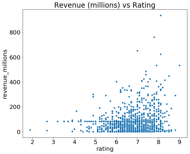
What's with the semicolon? It's not a syntax error, just a way to hide the <matplotlib.axes._subplots.AxesSubplot at 0x26613b5cc18> output when plotting in Jupyter notebooks.
If we want to plot a simple Histogram based on a single column, we can call plot on a column:
movies_df['rating'].plot(kind='hist', title='Rating');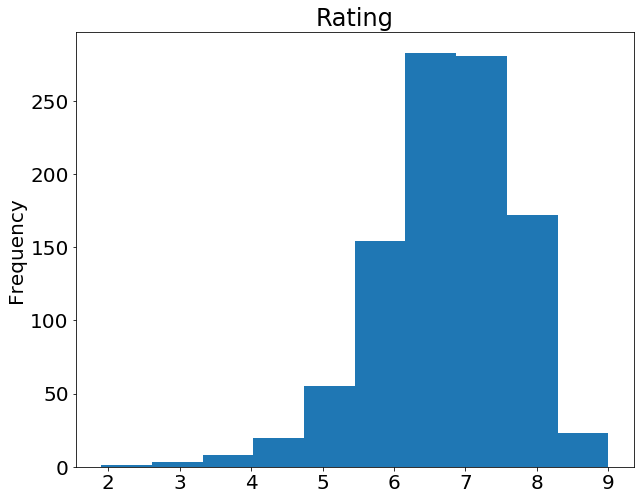
Do you remember the .describe() example at the beginning of this tutorial? Well, there's a graphical representation of the interquartile range, called the Boxplot. Let's recall what describe() gives us on the ratings column:
movies_df['rating'].describe()count 1000.000000
mean 6.723200
std 0.945429
min 1.900000
25% 6.200000
50% 6.800000
75% 7.400000
max 9.000000
Name: rating, dtype: float64Using a Boxplot we can visualize this data:
movies_df['rating'].plot(kind="box");

By combining categorical and continuous data, we can create a Boxplot of revenue that is grouped by the Rating Category we created above:
movies_df.boxplot(column='revenue_millions', by='rating_category');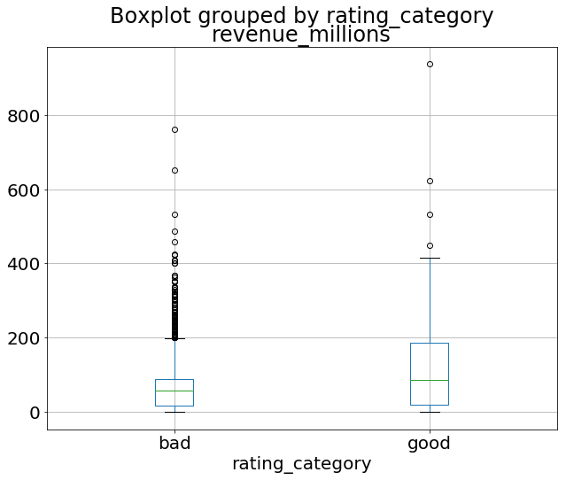
That's the general idea of plotting with pandas. There's too many plots to mention, so definitely take a look at the plot() docs here for more information on what it can do.
Wrapping up
Exploring, cleaning, transforming, and visualization data with pandas in Python is an essential skill in data science. Just cleaning wrangling data is 80% of your job as a Data Scientist. After a few projects and some practice, you should be very comfortable with most of the basics.
To keep improving, view the extensive tutorials offered by the official pandas docs, follow along with a few Kaggle kernels, and keep working on your own projects!
Resources
Applied Data Science with Python — Coursera
Covers an intro to Python, Visualization, Machine Learning, Text Mining, and Social Network Analysis in Python. Also provides many challenging quizzes and assignments to further enhance your learning.
Complete SQL Bootcamp — Udemy
An excellent course for learning SQL. The instructor explains everything from beginner to advanced SQL queries and techniques, and provides many exercises to help you learn.
Meet the Authors

Data Scientist and writer, currently working as a Data Visualization Analyst at Callisto Media


Lead data scientist and machine learning developer at smartQED, and mentor at the Thinkful Data Science program.