
Solar Energy Engineer, Ph.D. Physics
Python NumPy Tutorial: An Applied Introduction for Beginners
You should already know:
- Some Linear Algebra. A good intro to Linear Algebra can be found in Andrew Ng's machine learning course.
- Basics of Python. See Treehouse for interactive lessons.
What is NumPy?
Numpy is an open-source library for working efficiently with arrays. Developed in 2005 by Travis Oliphant, the name stands for Numerical Python. As a critical data science library in Python, many other libraries depend on it.
Why is NumPy so popular?
NumPy is extremely popular because it dramatically improves the ease and performance of working with multidimensional arrays.
Some of Numpy's advantages:
- Mathematical operations on NumPy’s ndarray objects are up to 50x faster than iterating over native Python lists using loops. The efficiency gains are primarily due to NumPy storing array elements in an ordered single location within memory, eliminating redundancies by having all elements be the same type and making full use of modern CPUs. The efficiency advantages become particularly apparent when operating on arrays with thousands or millions of elements, which are pretty standard within data science.
- It offers an Indexing syntax for easily accessing portions of data within an array.
- It contains built-in functions that improve quality of life when working with arrays and math, such as functions for linear algebra, array transformations, and matrix math.
- It requires fewer lines of code for most mathematical operations than native Python lists.
Best place to get more info
The online documentation (https://numpy.org/doc/) is a great place to look for further information on topics introduced in this article. The documentation goes into more detail than this introduction and is continually updated with evolving best practices.
When should you start using NumPy?
NumPy would be a good candidate for the first library to explore after gaining basic comfort with the Python environment. After NumPy, the next logical choices for growing your data science and scientific computing capabilities might be SciPy and pandas. In short, learn Python, then NumPy, then SciPy, or pandas.
What's the relationship between NumPy, SciPy, Scikit-learn, and Pandas?
- NumPy provides a foundation on which other data science packages are built, including SciPy, Scikit-learn, and Pandas.
- SciPy provides a menu of libraries for scientific computations. It extends NumPy by including integration, interpolation, signal processing, more linear algebra functions, descriptive and inferential statistics, numerical optimizations, and more.
- Scikit-learn extends NumPy and SciPy with advanced machine-learning algorithms.
- Pandas extends NumPy by providing functions for exploratory data analysis, statistics, and data visualization. It can be thought of as Python's equivalent to Microsoft Excel spreadsheets for working with and exploring tabular data (tutorial).
An Alternative to MATLAB?
Many readers will likely be familiar with the commercial scientific computing software MATLAB. When used together with other Python libraries like Matplotlib, NumPy can be considered as a fully-fledged alternative to MATLAB's core functionality.
Python is quite an attractive alternative to MATLAB for the following reasons:
- Python is open-source, which means that you have the option of inspecting the source code yourself.
- Access the vast and ever-growing possibilities open to Python users.
- Unlike MATLAB, Python and Numpy are free. No further explanation is needed!
Installation
To check if you already have NumPy installed in your Python installation (it most likely is), run the following command:
import numpy as npIf no error message is returned, that's a good sign NumPy is already available. If you get an error message like
ModuleNotFoundError: No module named 'numpy'
This probably means that NumPy needs to be installed first. If you use the pip Python package manager, the required command is 'pip install numpy'. If you need more detailed installation instructions, refer to https://numpy.org/.
List of useful NumPy functions
NumPy has numerous useful functions. You can see the full list of functions in the NumPy docs. As an overview, here are some of the most popular and useful ones to give you a sense of what NumPy can do. We will cover many of them in this tutorial.
- Array Creation: arange, array, copy, empty, empty_like, eye, fromfile, fromfunction, identity, linspace, logspace, mgrid, ogrid, ones, ones_like, r_, zeros, zeros_like
- Conversions: ndarray.astype, atleast_1d, atleast_2d, atleast_3d, mat
- Manipulations: array_split, column_stack, concatenate, diagonal, dsplit, dstack, hsplit, hstack, ndarray.item, newaxis, ravel, repeat, reshape, resize, squeeze, swapaxes, take, transpose, vsplit, vstack
- Questions: all, any, nonzero, where
- Ordering: argmax, argmin, argsort, max, min, ptp, searchsorted, sort
- Operations: choose, compress, cumprod, cumsum, inner, ndarray.fill, imag, prod, put, putmask, real, sum
- Basic Statistics: cov, mean, std, var
- Basic Linear Algebra: cross, dot, outer, linalg.svd, vdot
Section 1: The basics
NumPy arrays
The NumPy array - an n-dimensional data structure - is the central object of the NumPy package.
A one-dimensional NumPy array can be thought of as a vector, a two-dimensional array as a matrix (i.e., a set of vectors), and a three-dimensional array as a tensor (i.e., a set of matrices).
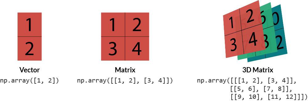
Need more than three dimensions? It's entirely possible to have arrays with many dimensions, including so many dimensions that it's no longer humanly possible to conceptualize them.
Array data types
An array can consist of integers, floating-point numbers, or strings. Within an array, the data type must be consistent (e.g., all integers or all floats).
Need an array with mixed data types? Consider using Numpy's record array format or pandas dataframes instead (see the Pandas tutorial).
In this article, we'll restrict our focus to conventional NumPy arrays consisting of a single data type.
Defining arrays
We can define NumPy arrays in a number of ways. We'll detail a few of the most common approaches below.
Using np.array()
To define an array manually, we can use the np.array() function. Below, we pass a list of two elements, each of which is a list containing two values. The result is a 2x2 matrix:
np.array([[1,2],[3,4]])array([[1, 2],
[3, 4]])It's as simple as that! Once we have our data in a NumPy array, a vast suite of computing possibilities becomes available. Much of this article is concerned with exploring these possibilities.
NumPy has numerous functions for generating commonly-used arrays without having to enter the elements manually. A few of those are shown below:
Defining arrays: np.arange()
The function np.arange() is great for creating vectors easily. Here, we create a vector with values spanning 1 up to (but not including) 5:
np.arange(1,5)array([1, 2, 3, 4])Defining arrays: np.zeros, np.ones, np.full
In many programming tasks, it can be useful to initialize a variable and then write a value to it later in the code. If that variable happens to be a NumPy array, a common approach would be to create it as an array with zeros in every element. We can do this using np.zeros(). Here, we create an array of zeros with three rows and one column.
np.zeros((3,1))array([[0.],
[0.],
[0.]])You can also initialize an array with ones instead of zeros:
np.ones((3, 1))array([[1.],
[1.],
[1.]])np.full() creates an array repeating a fixed value (defaults to zero). Here we create a 2x3 array with the number 7 in each element:
np.full((2,3),7)array([[7, 7, 7],
[7, 7, 7]])Making arrays in this way is also helpful for appending columns or rows to an existing arrays, which will be covered a little later.
Array shape
All arrays have a shape accessible using .shape.
For example, let's get the shape of a vector, matrix, and tensor.
vector = np.arange(5)
print("Vector shape:", vector.shape)
matrix = np.ones([3, 2])
print("Matrix shape:", matrix.shape)
tensor = np.zeros([2, 3, 3])
print("Tensor shape:", tensor.shape)Vector shape: (5,)
Matrix shape: (3, 2)
Tensor shape: (2, 3, 3)The shape of the vector is one-dimensional. The first number in its shape is the number of elements (or rows). For the matrix, .shape tells us we have three rows and two columns. The tensor is slightly different. The first number is how many matrices/slices we have. The second gives the number of rows. The third provides the number of columns.
If you're familiar with pandas, you might have noticed that the syntax for the number of rows and columns is strikingly similar to the equivalent in pandas. As we continue to explore NumPy arrays, you may notice many more similarities.
If we print the tensor, we can see it's representation as a list of 3x3 matrices:
tensorarray([[[0., 0., 0.],
[0., 0., 0.],
[0., 0., 0.]],
[[0., 0., 0.],
[0., 0., 0.],
[0., 0., 0.]]])Reshaping arrays
We can reshape an array into any compatible dimensions using .reshape .
For example, say we want a 3x3 matrix where each element is incremented from 1 to 9. Easy:
arr = np.arange(1, 10)
print(arr, '\n')
# Reshape to 3x3 matrix
arr = arr.reshape(3, 3)
print(arr, '\n')
# Reshape back to the original size
arr = arr.reshape(9)
print(arr)[1 2 3 4 5 6 7 8 9]
[[1 2 3]
[4 5 6]
[7 8 9]]
[1 2 3 4 5 6 7 8 9]Numpy can try to infer one of the dimensions if you use -1. You will still need to have precisely the correct number of digits for the inference to work.
arr = np.arange(1, 10).reshape(3, -1)
print(arr)[[1 2 3]
[4 5 6]
[7 8 9]]Reading data from a file into an array
Usually, data sets are too large to define manually. Instead, the most common use case is to import data from a data file into a NumPy array.
As an example, let's take some publicly-available data from the U.S. Energy Information Administration. The dataset we'll explore contains information on electricity generation in the USA from a range of sources. You can download the file, MER_T07_02A.csv, here: https://www.eia.gov/totalenergy/data/browser/csv.php?tbl=T07.02A.
Because the data file is a CSV file, we'll use the csv module to import the data. It's worth noting that NumPy also has functions to read other types of data files directly into NumPy arrays, such as np.genfromtxt() for text files.
Here we're just reading the CSV file row-by-row, appending to a list, and then converting to a NumPy array:
import csv
data = []
with open('MER_T07_02A.csv', 'r') as csvfile:
file_reader = csv.reader(csvfile, delimiter=',')
for row in file_reader:
data.append(row)
data = np.array(data) #convert the list of lists to a NumPy arrayNote
When you get familiar with pandas, a simpler option would be to use read_csv(). See our pandas tutorial for more info.
We now have our data stored in a NumPy array that we've named data. For much of the remainder of this article, we'll be exploring how NumPy's functionality can be used to manipulate and gain insights into this data.
First, we'll explore some attributes of the array. One thing that we may want to know about an array is its dimensions:
data.shape(8399, 6)For this two-dimensional array, we have 8230 rows and 6 columns of data.
Another property of a NumPy array that we may wish to know is its data type. This information is stored in the dtype attribute. Calling dtype reveals that our array is made up of strings:
data.dtype.typenumpy.str_Saving
When we are ready to save our data, we can use the save function.
np.save(open('data.npy', 'wb'), data) # Saves data to a binary file with the .npy extensionIndexing
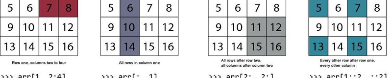
At some point, it will become necessary to index (select) subsets of a NumPy array. For instance, you might want to plot one column of data or perform a manipulation of that column. NumPy uses the same indexing notation as MATLAB.
Basics of indexing notation
- Commas separate axes of an array.
- Colons mean "through". For example, x[0:4] means the first 5 rows (rows 0 through 4) of x.
- Negative numbers mean "from the end of the array." For example, x[-1] means the last row of x.
- Blanks before or after colons means "the rest of". For example, x[3:] means the rest of the rows in x after row 3. Similarly, x[:3] means all the rows up to row 3. x[:] means all rows of x.
- When there are fewer indices than axes, the missing indices are considered complete slices. For example, in a 3-axis array, x[0,0] means all data in the 3rd axis of the 1st row and 1st column.
- Dots "..." mean as many colons as needed to produce a complete indexing tuple. For example, x[1,2,...] is the same as x[1,2,:,:,:].
In the following code, we'll explore some useful examples of selecting subsets from an array.
Examples
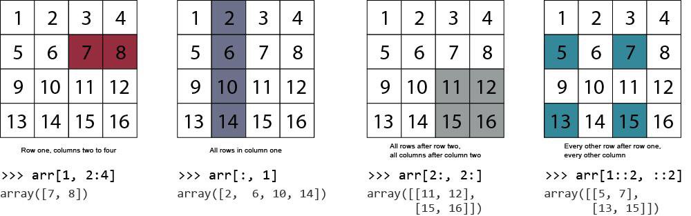
Indexing example 1: Colons and commas
Let's say we are interested in the first ten rows in the 4th column. We can use the following syntax to index this array section: __array[start_row:end_row, col]__
data[0:10,4]array(['Description', 'Electricity Net Generation From Coal, All Sectors',
'Electricity Net Generation From Coal, All Sectors',
'Electricity Net Generation From Coal, All Sectors',
'Electricity Net Generation From Coal, All Sectors',
'Electricity Net Generation From Coal, All Sectors',
'Electricity Net Generation From Coal, All Sectors',
'Electricity Net Generation From Coal, All Sectors',
'Electricity Net Generation From Coal, All Sectors',
'Electricity Net Generation From Coal, All Sectors'], dtype='<U80')The first row is the header for the column. Column 4 contains a description of energy sectors.
Indexing example 1: Colons as *all* rows or columns
A colon can also denote all rows, or all columns. Here, we index all rows of column 4.
data[:,4]array(['Description', 'Electricity Net Generation From Coal, All Sectors',
'Electricity Net Generation From Coal, All Sectors', ...,
'Electricity Net Generation Total (including from sources not shown), All Sectors',
'Electricity Net Generation Total (including from sources not shown), All Sectors',
'Electricity Net Generation Total (including from sources not shown), All Sectors'],
dtype='<U80')Indexing example 3: Subset of columns
We can use the same format for any dimension of an array. The general syntax is: array[start_row:end_row, start_col:end_col]. The following indexes all rows and the second column up to (but not including) the 4th column:
data[:,2:4]array([['Value', 'Column_Order'],
['135451.32', '1'],
['154519.994', '1'],
...,
['334166.94', '13'],
['314400.63', '13'],
['301776.141', '13']], dtype='<U80')Indexing example 4: Explicitly specifying column numbers
What if the columns we need are not next to each other? Instead of indexing a range of columns, it can be useful to specify them explicitly. To explicitly specify particular columns, we just include them in a list. Let's index the five rows after the header, selecting only columns 2 and 3. This time, we'll write the output to a new array named subset that we can re-use in the following example.
subset = data[1:6, [2,3]]
subsetarray([['135451.32', '1'],
['154519.994', '1'],
['185203.657', '1'],
['195436.666', '1'],
['218846.325', '1']], dtype='<U80')Indexing example 5: Mask arrays
Another convenient way to index certain sections of a NumPy array is to use a mask array. A mask array, also known as a logical array, contains boolean elements (i.e. True or False). Indexing of a given array element is determined by the value of the mask array's corresponding element.
First, we define a NumPy array of True/False values, where the True values are the ones we want to keep. Then we mask the subset array from the previous example. The result is retaining only the rows that correspond to elements that are True in the mask array.
mask_array = np.array([False, True, False, True, True])
subset[mask_array]array([['154519.994', '1'],
['195436.666', '1'],
['218846.325', '1']], dtype='<U80')As you can see, the mask array retained the rows corresponding to True and the excluded the ones corresponding to False. It is worth noting that a similar approach is used for indexing pandas dataframes.
Masking is a powerful tool that allows us to index elements based on logical expressions. We'll make good use of in the case study later in the article.
Concatenating
NumPy also provides useful functions for concatenating (i.e., joining) arrays. Let's say we wanted to restrict our attention to the first and the last three rows of our dataset. First, we'll define new sub-arrays as follows:
array_start = data[:3,:]
array_startarray([['MSN', 'YYYYMM', 'Value', 'Column_Order', 'Description', 'Unit'],
['CLETPUS', '194913', '135451.32', '1',
'Electricity Net Generation From Coal, All Sectors',
'Million Kilowatthours'],
['CLETPUS', '195013', '154519.994', '1',
'Electricity Net Generation From Coal, All Sectors',
'Million Kilowatthours']], dtype='<U80')array_end = data[-3:,:]
array_endarray([['ELETPUS', '202009', '334166.94', '13',
'Electricity Net Generation Total (including from sources not shown), All Sectors',
'Million Kilowatthours'],
['ELETPUS', '202010', '314400.63', '13',
'Electricity Net Generation Total (including from sources not shown), All Sectors',
'Million Kilowatthours'],
['ELETPUS', '202011', '301776.141', '13',
'Electricity Net Generation Total (including from sources not shown), All Sectors',
'Million Kilowatthours']], dtype='<U80')To concatenate these arrays we can use np.vstack, where the v denotes vertical, or row-wise, stacking of the sub-arrays:
np.vstack((array_start, array_end))array([['MSN', 'YYYYMM', 'Value', 'Column_Order', 'Description', 'Unit'],
['CLETPUS', '194913', '135451.32', '1',
'Electricity Net Generation From Coal, All Sectors',
'Million Kilowatthours'],
['CLETPUS', '195013', '154519.994', '1',
'Electricity Net Generation From Coal, All Sectors',
'Million Kilowatthours'],
['ELETPUS', '202009', '334166.94', '13',
'Electricity Net Generation Total (including from sources not shown), All Sectors',
'Million Kilowatthours'],
['ELETPUS', '202010', '314400.63', '13',
'Electricity Net Generation Total (including from sources not shown), All Sectors',
'Million Kilowatthours'],
['ELETPUS', '202011', '301776.141', '13',
'Electricity Net Generation Total (including from sources not shown), All Sectors',
'Million Kilowatthours']], dtype='<U80')Here we've stacked the first three rows and last three rows on top of each other.
The horizontal counterpart of np.vstack() is np.hstack(), which combines sub-arrays column-wise. For higher dimensional joins, the most common function is np.concatenate(). The syntax for this function is similar to the 2D versions, with the additional requirement of specifying the axis along which concatenation should be performed.
Calling np.concatenate((array_start, array_end), axis = 0) would generate identical output to using np.vstack(). Axis=1 would generate identical output to using np.hstack().
Splitting
The opposite of concatenating (i.e., joining) arrays is splitting them. To split an array, NumPy provides the following commands:
hsplit: splits along the horizontal axisvsplit: splits along the vertical axisdsplit: Splits an array along the 3rd axis (depth)array_split: lets you specify the axis to use in splitting
Adding/Removing Elements
NumPy provides several functions for adding or deleting data from an array:
resize: Returns a new array with the specified shape, with zeros as placeholders in all the new cells.append: Adds values to the end of an arrayinsert: Adds values in the middle of an arraydelete: Returns a new array with given data removedunique: Finds only the unique values of an array
Sorting
There are several useful functions for sorting array elements. Some of the available sorting algorithms include quicksort, heapsort, mergesort, and timesort.
For example, here's how you'd merge sort the columns of an array:
a = np.array([[3,8,1,2], [9,5,4,8]])
np.sort(a, axis=1, kind='mergesort') # Sort by columnarray([[1, 2, 3, 8],
[4, 5, 8, 9]])No Copy vs. Shallow Copy vs. Deep Copy
A common source of confusion NumPy beginners is knowing when data is and isn't copied into a new object.
No copy: function calls and assignments:
print(id(a))
# Object "b" points to object "a". No new object is created.
b = a
# Python passes objects as references. No copy is made.
def f(x):
print(id(x))
f(b)2270228861696
2270228861696Notice the id of b is the same as a, even if it's passed into a function.
View/Shallow Copy: Arrays that share some data. The view method creates an object looking at the same data. Slicing an array returns a view of that array.
# View
a = b.view()
# The shape of b doesn't change
a = a.reshape((4, 2))
# Slice
# a[:] is a view of "a".
a[:] = 5Deep copy: Use the copy method to make a complete copy of an array and all its data.
c = a.copy()The copy() method creates the new array object c that is identical to a.
Section 2: Must-know tools
Let's now look at three NumPy tools that are especially handy in data science applications: broadcasting, vectorization, and pseudo-random number generation. For this section, we'll put our electricity dataset aside in favor of even more straightforward examples.
Broadcasting

Broadcasting is a process performed by NumPy that allows mathematical operations to work with objects that don't necessarily have compatible dimensions.
Let's explore broadcasting using some examples.
Broadcasting example 1: Adding a scalar to a matrix
Suppose we would like to add 1 to each element of a 2x2 array. With NumPy arrays, it is as simple as defining the array and adding 1:
array_a = np.array([[1, 2],
[3, 4]])
array_a + 1array([[2, 3],
[4, 5]])Keep in mind that any university linear algebra instructor would be furious if you even mentioned the notion of adding a scalar to a matrix. And not without reason: it isn't a mathematically valid operation.
However, what NumPy is doing in the background is valid. NumPy creates a second array with value 1 for all elements (depicted by transparent blocks in the above figure). NumPy then adds the second array to the first one.
In other words, NumPy has broadcast the scalar to a new array of appropriate dimensions to perform the computation.
Numpy accomplishes broadcasting in a very computationally efficient way, which is one of the key advantages of using broadcasting in your code. Broadcasting may also make your code simpler and more readable.
Let's look at some more examples.
Broadcasting example 2: Multiplying a matrix by a scalar
Multiplication works the same way as addition.
array_a * 2array([[2, 4],
[6, 8]])Broadcasting example 3:
We can use broadcasting in cases beyond just overcoming the dimensional mismatch between a scalar and an array. NumPy can also broadcast arrays to enable computations with other arrays.
Let's say that each row of array_a, defined above, is a collection of two objects. The coordinates of the first object (first row of array_a) is located at (x = 1, y = 2), and the other object (second row of array_a) is located at (x = 3, y = 4). To find the coordinates of both objects if they both were translated by 3 units in the x direction and 1 unit in the y direction, all we would need to do is add (3, 1) to array_a:
array_a + np.array([3, 1])array([[4, 3],
[6, 5]])This time, NumPy created a second 2x2 matrix (in the background), with both rows equal to [3, 1], to perform the operation. In other words, Numpy broadcasts the 1x2 array to an array appropriate to perform the operation with the 2x2 array.
The operation is equivalent to the one depicted in the second row of the above figure.
For even more examples of broadcasting, the best place to look is the documentation.
Let's now move on to another essential tool: vectorization.
Vectorization
Vectorization is the process of modifying code to utilize array operation methods. Array operations can be computed internally by NumPy using a lower-level language, which leads to many benefits:
- Vectorized code tends to execute much faster than equivalent code that uses loops (such as for-loops and while-loops). Usually a lot faster. Therefore, vectorization can be very important for machine learning, where we often work with large datasets
- Vectorized code can often be more compact. Having fewer lines of code to write can potentially speed-up the code-writing process, make code more readable, and reduce the risk of errors
Vectorization Example 1
Let's consider a problem where we have two one-dimensional arrays, a and b, and we need to multiply each element in a with the corresponding element in b.
First we'll define some arbitrary values for a and b:
a = np.arange(1,51)
b = np.arange(51,101)
print("array a:", a)
print("\narray b:", b)array a: [ 1 2 3 4 5 6 7 8 9 10 11 12 13 14 15 16 17 18 19 20 21 22 23 24
25 26 27 28 29 30 31 32 33 34 35 36 37 38 39 40 41 42 43 44 45 46 47 48
49 50]
array b: [ 51 52 53 54 55 56 57 58 59 60 61 62 63 64 65 66 67 68
69 70 71 72 73 74 75 76 77 78 79 80 81 82 83 84 85 86
87 88 89 90 91 92 93 94 95 96 97 98 99 100]First we'll multiply the elements using a simple Python loop. This is the non-vectorized version:
def non_vectorized_output(a, b):
output = []
for j in range(len(a)):
output.append(a[j]*b[j])
return outputCalculating the speed up
Using Jupyter's magic timeit command, we can calculate how long it takes to run this function over many executions:
nv_time = %timeit -o non_vectorized_output(a, b)21.4 µs ± 506 ns per loop (mean ± std. dev. of 7 runs, 10000 loops each)The %timeit -o command will run a function over many executions and store the timing results in a variable. You can also just run %timeit non_vectorized_output(a, b) if you don't care about storing the result in a variable.
Now we'll use the multiplication operator between arrays to allow Numpy to handle the multiplication instead. This is the vectorized version:
def vectorized_output(a, b):
return a * bv_time = %timeit -o vectorized_output(a, b)701 ns ± 14.3 ns per loop (mean ± std. dev. of 7 runs, 1000000 loops each)As you can see, the looping in the non-vectorized version is performed in pure Python (i.e., without using NumPy) with a for-loop. Although it would be challenging to make this non-vectorized code function any more compactly, it still occupies three more lines of code than the vectorized version. This compactness is in part because the looping in the vectorized version happens in the background.
It's clear that vectorized code is more compact, but what is the difference in computation time? Let's print the results in a way that's easier to read:
print('Non-vectorized version:', f'{1E6 * nv_time.average:0.2f}', 'microseconds per execution, average')
print('Vectorized version:', f'{1E6 * v_time.average:0.2f}', 'microseconds per execution, average')
print('Computation was', "%.0f" % (nv_time.average / v_time.average), 'times faster using vectorization')Non-vectorized version: 21.40 microseconds per execution, average
Vectorized version: 0.70 microseconds per execution, average
Computation was 31 times faster using vectorizationVectorization example 2
In this second example, we'll evaluate a set of linear expressions. Again, this task could be accomplished either using for-loops or using vectorized code.
In this case, the vectorized version will use matrix multiplication to evaluate the linear expressions. If you're familiar with machine learning (ML), the next paragraph will provide some context about when you might encounter this in ML.
Machine Learning context
Let's imagine a machine learning problem where we use a linear regression algorithm to model the cost of electricity.
Let's denote our model features as $x_1, x_2 ... x_{n}$. Features could represent things like the amount of available wind energy, the current gas price, and the current load on the grid.
After we train the algorithm, we obtain model parameters, $\theta_0,\theta_1,\theta_2...\theta_{n}$. These model parameters constitute the weights that should be used for each feature.
For instance, $x_2$ might represent the price of gas. The model might find that gas prices are particularly decisive in determining the price of electricity. The corresponding weight of $\theta_2$ would then be expected to be much larger in magnitude than other weights for less important features. The result (hypothesis/prediction) returned by our linear regression model for a given set of $x$ is a linear expression:
$$ h=\theta_0 + x_1 \theta_1 + x_2 \theta_2 + ... + x_{n} \theta_{n}$$
Furthermore, let's assume we have a set of $m$ test examples. In other words, we have $m$ sets of $x$ for which we would like to obtain the model's prediction. The linear expression, $h$, is to be calculated for each of the test examples. There will be a total of $m$ individual hypothesis outputs.
As we'll see below, this can all be calculated concisely using one vectorized statement. To start, we'll define some arbitrary values for the array of test examples ($x$), and the vector of model parameters ($\theta$, theta).
In an ML problem, our model parameters would be calculated as an output of an optimization procedure. For the sake of this example, we'll just use arbitrary values.
First, define a 10x4 array (x) in which each row is a training set. Here, $m = 10$ and $n = 4$:
x = np.arange(1,41).reshape(10,4)
print('x:\n', x)x:
[[ 1 2 3 4]
[ 5 6 7 8]
[ 9 10 11 12]
[13 14 15 16]
[17 18 19 20]
[21 22 23 24]
[25 26 27 28]
[29 30 31 32]
[33 34 35 36]
[37 38 39 40]]x is now a range of 40 numbers reshaped to be 10 rows by 4 columns.
Now, add a column of ones to represent $x_0$, known in machine learning as the bias term. x is now a 10x5 array:
ones = np.full((10,1),1)
x = np.hstack((ones,x))
print('x:\n', x)x:
[[ 1 1 2 3 4]
[ 1 5 6 7 8]
[ 1 9 10 11 12]
[ 1 13 14 15 16]
[ 1 17 18 19 20]
[ 1 21 22 23 24]
[ 1 25 26 27 28]
[ 1 29 30 31 32]
[ 1 33 34 35 36]
[ 1 37 38 39 40]]Using np.full, we created a 10x1 array full of ones then horizontally stacked it (np.hstack) to the front of x.
Now let's initialize our model parameters as a 5x1 array
theta = np.arange(1,6).reshape(5,1)
print('theta:\n', theta)theta:
[[1]
[2]
[3]
[4]
[5]]Armed with our matrix $x$ and vector $\theta$, we'll proceed to define vectorized and non-vectorized versions of evaluating the linear expressions to compare the computation time.
#Non-vectorized version
def non_vectorized_output(x, theta):
h = []
for i in range(x.shape[0]):
total = 0
for j in range(x.shape[1]):
total = total + x[i, j] * theta[j, 0]
h.append(total)
return h
#Vectorized version
def vectorized_output(x, theta):
h = np.matmul(x, theta) # NumPy's matrix multiplication function
return hnv_time = %timeit -o non_vectorized_output(x, theta)34.7 µs ± 410 ns per loop (mean ± std. dev. of 7 runs, 10000 loops each)v_time = %timeit -o vectorized_output(x, theta)1.58 µs ± 9.66 ns per loop (mean ± std. dev. of 7 runs, 1000000 loops each)print('Non-vectorized version:', f'{1E6 * nv_time.average:0.2f}', 'microseconds per execution, average')
print('Vectorized version:', f'{1E6 * v_time.average:0.2f}', 'microseconds per execution, average')
print('Computation was', "%.0f" % (nv_time.average / v_time.average), 'times faster using vectorization')Non-vectorized version: 34.69 microseconds per execution, average
Vectorized version: 1.58 microseconds per execution, average
Computation was 22 times faster using vectorizationNote that in both examples, NumPy's vectorized calculations significantly outperformed native Python calculations using loops. The improved performance is substantial.
However, vectorization does have potential disadvantages. Vectorized code can be less intuitive to those who do not know how to read it. It can also be more memory intensive. The skill of knowing how much vectorization to use in your code is something that you'll develop with experience. The decision will always need to be made based on the nature of the application in question.
Pseudo-random number generation
Before we finish this section, there is one more NumPy functionality that we should cover: pseudo-random number generation.
Being able to generate pseudo-random numbers is often necessary in data science applications. Examples include modeling system noise and Monte Carlo simulations.
Below we'll see how to generate random numbers (x) from two commonly encountered probability distributions: the uniform distribution and the normal (Gaussian) distribution.
For this, we'll import matplotlib and set some default plotting styles:
import matplotlib.pyplot as plt
import matplotlib
# Set some default plotting parameters
matplotlib.rcParams.update({'font.size': 16,
'figure.figsize': [10, 6],
'lines.markersize': 6})For the Uniform, we'll generate a NumPy array with 1000 samples randomly selected from a uniform distribution using random.rand.
For the Normal, we'll generate a NumPy array with 1000 samples from a normal distribution centred at 5 with a standard deviation of 3 using random.normal:
uniform_data = np.random.rand(1000)
normal_data = np.random.normal(loc=5, scale=3.0, size=1000)Here's a plot of the histograms for the Uniform data (first subplot) and the Normal data (second subplot):
fig = plt.figure() # Define the figure
ax1 = fig.add_subplot(1,2,1) # define location of first subplot
ax1.hist(x=uniform_data, bins='auto',alpha=0.7, rwidth=0.85)
ax1.set_title("Uniform Distribution")
ax2 = fig.add_subplot(1,2,2) # define location of second subplot
ax2.hist(x=normal_data, bins='auto', alpha=0.7, rwidth=0.7)
ax2.set_title("Normal Distribution")
ax1.set_ylabel('Frequency')
ax1.set_xlabel('x')
ax2.set_xlabel('x')
plt.show()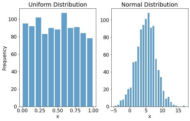
As we'd expect, uniform distribution's random values are more or less equally spaced between zero and one. By contrast, the values from the normal distribution take on the characteristic bell-curve shape.
We can now use the sets of random numbers we've just generated in further computations, but we'll leave that for another time. To wrap up this article, let's put everything we learned together using our electricity dataset.
Section 3: Putting it all together
Now that we know the basics of NumPy, broadcasting, and vectorization, we have everything we need to start diving into the electricity data that we imported at the start of this article.
Let's assume we'd like to understand how the USA's electricity generation has changed over time.
Viewing the data
Using what we've learned about indexing, we can start by separating the column labels from the rest of the data.
header = data[0,:] # create a new NumPy array containing the column labels
data = data[1:,:] # remove the header from the rest of the data
print('Header:\n',header, '\n\nFirst two rows:\n', data[:2,:])Header:
['MSN' 'YYYYMM' 'Value' 'Column_Order' 'Description' 'Unit']
First two rows:
[['CLETPUS' '194913' '135451.32' '1'
'Electricity Net Generation From Coal, All Sectors'
'Million Kilowatthours']
['CLETPUS' '195013' '154519.994' '1'
'Electricity Net Generation From Coal, All Sectors'
'Million Kilowatthours']]To understand how electricity generation has changed with time, we'll need to pay attention to column 1 (date), column 2 (energy generated), and column 4 (description).
In this dataset, rows containing monthly data express date in the format 'YYYYMM'. Rows containing annual data express the date in the format 'YYYY13'.
Our dataset happens to contain generation data from many different energy sources, so let's determine which energy sources are present in this dataset by inspecting the descriptions (column 4).
The np.unique() function makes it easy to see all energy sources. As the name suggests, it will return all unique values in the array.
np.unique(data[:,4])array(['Electricity Net Generation From Coal, All Sectors',
'Electricity Net Generation From Conventional Hydroelectric Power, All Sectors',
'Electricity Net Generation From Geothermal, All Sectors',
'Electricity Net Generation From Hydroelectric Pumped Storage, All Sectors',
'Electricity Net Generation From Natural Gas, All Sectors',
'Electricity Net Generation From Nuclear Electric Power, All Sectors',
'Electricity Net Generation From Other Gases, All Sectors',
'Electricity Net Generation From Petroleum, All Sectors',
'Electricity Net Generation From Solar, All Sectors',
'Electricity Net Generation From Waste, All Sectors',
'Electricity Net Generation From Wind, All Sectors',
'Electricity Net Generation From Wood, All Sectors',
'Electricity Net Generation Total (including from sources not shown), All Sectors'],
dtype='<U80')This dataset contains information from a total of 13 categories of energy sources.
Extracting wind energy data
Next, we'll extract a subset containing just the wind energy generation data. We'll be making extensive use of indexing with mask arrays, which we looked at earlier.
Let's start by retaining only the rows that contain wind data. First, we'll create a mask array that contains True entries for every row of wind data:
mask_array = (data[:,4] == 'Electricity Net Generation From Wind, All Sectors')
mask_arrayarray([False, False, False, ..., False, False, False])What this mask array essentially says is "get all rows where column four equals 'Electricity Net Generation...'"
Now we can use it to mask our data:
wind_data = data[mask_array]
wind_dataarray([['WYETPUS', '194913', 'Not Available', '12',
'Electricity Net Generation From Wind, All Sectors',
'Million Kilowatthours'],
['WYETPUS', '195013', 'Not Available', '12',
'Electricity Net Generation From Wind, All Sectors',
'Million Kilowatthours'],
['WYETPUS', '195113', 'Not Available', '12',
'Electricity Net Generation From Wind, All Sectors',
'Million Kilowatthours'],
...,
['WYETPUS', '202009', '23176.032', '12',
'Electricity Net Generation From Wind, All Sectors',
'Million Kilowatthours'],
['WYETPUS', '202010', '29418.649', '12',
'Electricity Net Generation From Wind, All Sectors',
'Million Kilowatthours'],
['WYETPUS', '202011', '33848.129', '12',
'Electricity Net Generation From Wind, All Sectors',
'Million Kilowatthours']], dtype='<U80')Did you notice that we used broadcasting to generate the mask array? Broadcasting allowed the generation of a new array based on the logical evaluation of whether each string element in an array was equal to a single string.
In the above output, we notice that some of the early rows contain the string _Not Available_ in the 'Value' column. _Not Available_ suggests that records only began later on. Let's exclude the rows for which no records exist:
wind_data = wind_data[wind_data[:,2] != 'Not Available']
wind_dataarray([['WYETPUS', '198301', '0.172', '12',
'Electricity Net Generation From Wind, All Sectors',
'Million Kilowatthours'],
['WYETPUS', '198302', '0.018', '12',
'Electricity Net Generation From Wind, All Sectors',
'Million Kilowatthours'],
['WYETPUS', '198303', '0.313', '12',
'Electricity Net Generation From Wind, All Sectors',
'Million Kilowatthours'],
...,
['WYETPUS', '202009', '23176.032', '12',
'Electricity Net Generation From Wind, All Sectors',
'Million Kilowatthours'],
['WYETPUS', '202010', '29418.649', '12',
'Electricity Net Generation From Wind, All Sectors',
'Million Kilowatthours'],
['WYETPUS', '202011', '33848.129', '12',
'Electricity Net Generation From Wind, All Sectors',
'Million Kilowatthours']], dtype='<U80')Note that the above code performed indexing using a mask array. For compactness, we didn't explicitly define the mask array as a separate object.
Now, let's retain only the annual data. In other words, keep only the rows where the value in column 1 ends with '13'. To do this, we use list comprehension (a pure Python formalism) to generate the mask array to perform the indexing.
annual_mask_array = np.array(([x[-2:] == '13' for x in wind_data[:,1]]))
wind_data = wind_data[annual_mask_array]
wind_data[:5]array([['WYETPUS', '198313', '2.668', '12',
'Electricity Net Generation From Wind, All Sectors',
'Million Kilowatthours'],
['WYETPUS', '198413', '6.49', '12',
'Electricity Net Generation From Wind, All Sectors',
'Million Kilowatthours'],
['WYETPUS', '198513', '5.762', '12',
'Electricity Net Generation From Wind, All Sectors',
'Million Kilowatthours'],
['WYETPUS', '198613', '4.189', '12',
'Electricity Net Generation From Wind, All Sectors',
'Million Kilowatthours'],
['WYETPUS', '198713', '3.541', '12',
'Electricity Net Generation From Wind, All Sectors',
'Million Kilowatthours']], dtype='<U80')We have now successfully isolated the annual wind data.
It is worth noting that it is straightforward to save a NumPy array to a text file using the np.savetxt() function.
Just for fun, let's save our results to a comma-delimited csv file. We will request that NumPy converts everything to a string format before exporting.
np.savetxt('wind.csv',wind_data, fmt = '%s', delimiter = ',')Now let's define a new NumPy array containing just the annual wind energy produced, which is contained in column two of our wind data array. We will convert information to a float data type:
energy = wind_data[:,2].astype(float)
energyarray([2.66800000e+00, 6.49000000e+00, 5.76200000e+00, 4.18900000e+00,
3.54100000e+00, 8.71000000e-01, 2.11204300e+03, 2.78860000e+03,
2.95095100e+03, 2.88752300e+03, 3.00582700e+03, 3.44710900e+03,
3.16425300e+03, 3.23406900e+03, 3.28803500e+03, 3.02569600e+03,
4.48799800e+03, 5.59326100e+03, 6.73733100e+03, 1.03542800e+04,
1.11874660e+04, 1.41437410e+04, 1.78105490e+04, 2.65891370e+04,
3.44499270e+04, 5.53631000e+04, 7.38861320e+04, 9.46522460e+04,
1.20176599e+05, 1.40821703e+05, 1.67839745e+05, 1.81655282e+05,
1.90718548e+05, 2.26992562e+05, 2.54302695e+05, 2.72667454e+05,
2.94906320e+05])Success! Now that we finally have the data of interest in an array of floating-point numbers, we can start taking advantage of some NumPy functions that can quickly and easily perform numerical operations on our array.
Mathematical functions
NumPy offers many mathematical functions that can be called with the syntax array.method(). For instance, if we wanted to compute the sum of all elements in the array, we could use the function array.sum():
print(f'Total wind energy generated in the USA since 1983 is {energy.sum()} Gigawatt-hours')Total wind energy generated in the USA since 1983 is 2235263.7029999997 Gigawatt-hoursEasy.
NumPy functions are also available to calculate things like the mean and standard deviation:
print(f'The average annual energy generated from wind is {energy.mean()} Gigawatt-hours, '
f'with a standard deviation of {100 * energy.std() / energy.mean():.2f}%')The average annual energy generated from wind is 60412.532513513506 Gigawatt-hours, with a standard deviation of 147.70%We can quickly answer many questions using these functions. Here are a couple more.
What was the maximum annual energy generated?
print(f'The highest recorded annual energy generated by wind power is {energy.max()} Gigawatt-hours')The highest recorded annual energy generated by wind power is 294906.32 Gigawatt-hoursAnd in what year did that occur?
index = energy.argmax() #this method returns the index of the maximum value in the array
print(f'The highest energy generation occured in the year {wind_data[index,1][:-2]}')The highest energy generation occured in the year 2019Fitting
Another important NumPy's capability is data fitting.
Let's say we wanted to predict the wind energy that will be generated the year after the period spanned by the dataset. A straightforward approach would be to fit a straight line to recent data and then extrapolate it out to the following year.
Although SciPy has some powerful fitting tools, in particular scipy.optimize.curve_fit(), it turns out that we don't need to move outside of NumPy to perform this fit.
Within NumPy, our options include np.linalg.lstsq() and NumPy's polynomial package. Here, we'll use the latter.
import numpy.polynomial.polynomial as poly
x = np.array([int(j[:4]) for j in wind_data[:,1]]) # Taking the first four digits of each entry in column 1 gives us the year
y = energy
poly_coeff= poly.polyfit(x[-10:], y[-10:],deg=1) # Get coefficients for a first-degree polynomial (straight line) fit for the most recent 10 years of data
fit = poly.polyval(x[-10:], poly_coeff) # Evaluate the fitted polynomial using the polynomial coefficients
fig, ax = plt.subplots() # Define a figure and axis on which to plot our data
ax.plot(x,y, 'ro', label = 'Data') # Plot the data
ax.plot(x[-10:], fit, 'b-', label='Linear fit to last 10 years') # Plot the fit
# Extrapolate
new_point = x[-1] + 1 # 1 year after the final datapoint
fit_new_point = poly.polyval(new_point, poly_coeff)
ax.plot(new_point, fit_new_point, 'gs', label=f'Predicted value in {str(new_point)}') # Plot the fit
# Label the axes
ax.set_xlabel('Year')
ax.set_ylabel('Net electricity generation \n from wind (Gwh)')
# Add a legend
plt.legend()
plt.show()
plt.close()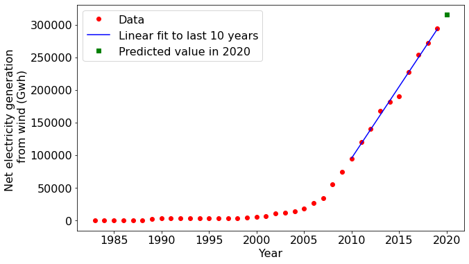
Notice that the matplotlib plotting commands accepted the NumPy arrays as inputs without a problem. You will find this compatibility with NumPy for quite a few other libraries in Python as well. The degree of compatibility reflects NumPy's core role in Python's overall data science and scientific computing capability.
One last plot...
Our plot above shows that the amount of wind-generated electricity has increased rapidly in the USA in the last ten years. But is this simply a consequence of the total electricity generation increasing? Or is the national grid fundamentally shifting toward wind energy? NumPy can help us answer this.
To make things more compact, we'll define a function to index certain rows from the primary dataset based on the earlier approach.
def index_energy_data(data, startyear, energy_label):
"""returns a NumPy array containing only rows with the specified energy_label in column 4,
that also contain energy data, and that also contain annual totals after the specified start year """
output = data[((data[:,4] == energy_label))]
output = output[((output[:,2] != 'Not Available'))]
output = output[np.array(([x[-2:] == '13' and int(x[:4]) >= startyear for x in output[:,1]]))]
energy = output[:,2].astype(float)
dates = np.array([int(j[:4]) for j in output[:,1]]) # Taking the first four digits of each entry in column 1 gives us the year
return energy, datesNow we'll apply this function to generate three arrays. Solar data was recorded from 1984 onwards, so we'll restrict all arrays to this timeframe:
energy_wind, dates = index_energy_data(data, 1984, energy_label = 'Electricity Net Generation From Wind, All Sectors')
energy_solar, dates = index_energy_data(data, 1984, energy_label = 'Electricity Net Generation From Solar, All Sectors')
energy_total, dates = index_energy_data(data, 1984, energy_label = 'Electricity Net Generation Total (including from sources not shown), All Sectors')Let's compute the contribution of wind, solar, and their combined contribution compared to the total energy generation in the USA:
wind_frac = 100 * energy_wind / energy_total
solar_frac = 100 * energy_solar / energy_total
combined_frac = 100 * (energy_solar + energy_wind) / energy_totalNow we have our data. Did you notice the use of vectorization and broadcasting above? Let's proceed to plotting the results:
# Prepare the plot
fig, ax = plt.subplots() # Define a figure and axis on which to plot our data
ax.plot(dates, wind_frac, 'ro-', label = 'Wind')
ax.plot(dates, solar_frac, 'bo-', label = 'Solar')
ax.plot(dates, combined_frac, 'ko-', label = 'Wind + Solar')
#Label the axes
ax.set_xlabel('Year')
ax.set_ylabel('Contribution to total USA \n electricity generation (%)')
#add a legend
plt.legend()
plt.show()
plt.close()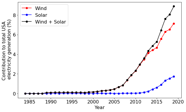
As this plot shows, the nature of the national grid is changing: there is a rapid change in the mix of electricity sources occurring.
To answer further questions, like what is driving this change, we would need a lot more data on the situation's social and economic factors. Rest assured, as soon as we get that data, NumPy would be up to the task of performing the required data manipulations!
Summary
In this article, we explored some of the handy computing tools offered by the NumPy library. We learned about the central object of the NumPy library - the NumPy array. We also learned how to create arrays in several ways: manually, using NumPy functions, and loading data from an external file into an array.
We explored two essential tools that are especially useful when dealing with large datasets: vectorization and broadcasting.
After that, we walked through an example using NumPy. We loaded a real set of data for historical electricity generation in the United States. We then analyzed the data to obtain an insight into the fundamental change in the electricity mix over time.
This article has provided you with an overview of NumPy's capabilities. You should now be ready to start using NumPy in your projects. Be sure to refer to the documentation (https://numpy.org/doc/) for specifics and other capabilities. Good luck!
Meet the Authors

Ricky holds a Ph.D. in physics and currently works in Silicon Valley, USA.

