

Quantitative Analyst
Python for Finance, Part I: Yahoo & Google Finance API, pandas, and matplotlib
Learn how to use pandas to call a finance API for stock data and easily calculate moving averages
LearnDataSci is reader-supported. When you purchase through links on our site, earned commissions help support our team of writers, researchers, and designers at no extra cost to you.
Updates
This article is in the process of being updated to reflect the new release of pandas_datareader (0.7.0), which should be out soon. Please check back later!
Motivation
Less than a decade ago, financial instruments called derivatives were at the height of popularity. Financial institutions around the world were trading billions of dollars of these instruments on a daily basis, and quantitative analysts were modeling them using stochastic calculus and the all mighty C++.
Fast forward nine years later and things have changed. The financial crisis has proven to be an as-to-yet derivatives-nemesis. Volumes have gone down and demand for C++ modeling has withered with them. But there is a new player in town… Python!
You should already know:
- Python fundamentals
- Some Pandas and Matplotlib
Learn both interactively through dataquest.io
Python has been gaining significant traction in the financial industry over the last years and with good reason. In this series of tutorials we are going to see how one can leverage the powerful functionality provided by a number of Python packages to develop and backtest a quantitative trading strategy.
In detail, in the first of our tutorials, we are going to show how one can easily use Python to download financial data from free online databases, manipulate the downloaded data and then create some basic technical indicators which will then be used as the basis of our quantitative strategy. To accomplish that, we are going to use one of the most powerful and widely used Python packages for data manipulation, pandas.
Getting the Data
Pandas and matplotlib are included in the more popular distributions of Python for Windows, such as Anaconda.
In case it's not included in your Python distribution, just simply use pip or conda install. Once installed, to use pandas, all one needs to do is import it. We will also need the pandas_datareader package (pip install pandas-datareader), as well as matplotlib for visualizing our results.
from pandas_datareader import data
import matplotlib.pyplot as plt
import pandas as pdHaving imported the appropriate tools, getting market data from a free online source, such as Yahoo Finance, is super easy. Since pandas has a simple remote data access for the Yahoo Finance API data, this is as simple as:
Update (4/14/18): Yahoo Finance API issue
Yahoo finance has changed the structure of its website and as a result the most popular Python packages for retrieving data have stopped functioning properly. Until this is resolved, we will be using Google Finance for the rest this article so that data is taken from Google Finance instead. We are using the ETF "SPY" as proxy for S&P 500 on Google Finance
Please note that there has been some issues with missing data in Google's API, as well as frequent, random errors that occur when pulling a lot of data.
# Define the instruments to download. We would like to see Apple, Microsoft and the S&P500 index.
tickers = ['AAPL', 'MSFT', '^GSPC']
# We would like all available data from 01/01/2000 until 12/31/2016.
start_date = '2010-01-01'
end_date = '2016-12-31'
# User pandas_reader.data.DataReader to load the desired data. As simple as that.
panel_data = data.DataReader('INPX', 'google', start_date, end_date)What does panel_data look like? data.DataReader returns a Panel object, which can be thought of as a 3D matrix. The first dimension consists of the various fields Yahoo Finance returns for a given instrument, namely, the Open, High, Low, Close and Adj Close prices for each date. The second dimension contain the dates. The third one contains the instrument identifiers.
Let's see what panel_data actually is by temporarily making it a dataframe and calling the top nine rows:
panel_data.to_frame().head(9)| Open | High | Low | Close | Volume | ||
|---|---|---|---|---|---|---|
| Date | minor | |||||
| 2010-01-04 | AAPL | 30.49 | 30.64 | 30.34 | 30.57 | 123432050.0 |
| MSFT | 30.62 | 31.10 | 30.59 | 30.95 | 38414185.0 | |
| SPY | 112.37 | 113.39 | 111.51 | 113.33 | 118944541.0 | |
| 2010-01-05 | AAPL | 30.66 | 30.80 | 30.46 | 30.63 | 150476004.0 |
| MSFT | 30.85 | 31.10 | 30.64 | 30.96 | 49758862.0 | |
| SPY | 113.26 | 113.68 | 112.85 | 113.63 | 111579866.0 | |
| 2010-01-06 | AAPL | 30.63 | 30.75 | 30.11 | 30.14 | 138039594.0 |
| MSFT | 30.88 | 31.08 | 30.52 | 30.77 | 58182332.0 | |
| SPY | 113.52 | 113.99 | 113.43 | 113.71 | 116074402.0 |
Preparing the Data
Let us assume we are interested in working with the Close prices which have been already been adjusted by Google finance to account for stock splits. We want to make sure that all weekdays are included in our dataset, which is very often desirable for quantitative trading strategies.
Of course, some of the weekdays might be public holidays in which case no price will be available. For this reason, we will fill the missing prices with the latest available prices:
# Getting just the adjusted closing prices. This will return a Pandas DataFrame
# The index in this DataFrame is the major index of the panel_data.
close = panel_data['Close']
# Getting all weekdays between 01/01/2000 and 12/31/2016
all_weekdays = pd.date_range(start=start_date, end=end_date, freq='B')
# How do we align the existing prices in adj_close with our new set of dates?
# All we need to do is reindex close using all_weekdays as the new index
close = close.reindex(all_weekdays)
# Reindexing will insert missing values (NaN) for the dates that were not present
# in the original set. To cope with this, we can fill the missing by replacing them
# with the latest available price for each instrument.
close = close.fillna(method='ffill')Initially, close contains all the closing prices for all instruments and all the dates that Google returned. Some of the week days might be missing from the data Google provides. For this reason we create a Series of all the weekdays between the first and last date of interest and store them in the all_weekdays variable. Getting all the weekdays is achieved by passing the freq=’B’ named parameter to the pd.date_range() function. This function return a DatetimeIndex which is shown below:
print(all_weekdays)
# DatetimeIndex(['2010-01-01', '2010-01-04', '2010-01-05', '2010-01-06',
# '2010-01-07', '2010-01-08', '2010-01-11', '2010-01-12',
# '2010-01-13', '2010-01-14',
# ...
# '2016-12-19', '2016-12-20', '2016-12-21', '2016-12-22',
# '2016-12-23', '2016-12-26', '2016-12-27', '2016-12-28',
# '2016-12-29', '2016-12-30'],
# dtype='datetime64[ns]', length=1826, freq='B')Aligning the original DataFrame with the new DatetimeIndex is accomplished by substitution of the initial DatetimeIndex of the close DataFrame. If any of the new dates were not included in the original DatetimeIndex, the prices for that date will be filled with NaNs. For this reason, we will fill any resulting NaNs with the last available price. The final, clean DataFrame is shown below:
close.head(10)| AAPL | MSFT | SPY | |
|---|---|---|---|
| 2010-01-01 | NaN | NaN | NaN |
| 2010-01-04 | 30.57 | 30.95 | 113.33 |
| 2010-01-05 | 30.63 | 30.96 | 113.63 |
| 2010-01-06 | 30.14 | 30.77 | 113.71 |
| 2010-01-07 | 30.08 | 30.45 | 114.19 |
| 2010-01-08 | 30.28 | 30.66 | 114.57 |
| 2010-01-11 | 30.02 | 30.27 | 114.73 |
| 2010-01-12 | 29.67 | 30.07 | 113.66 |
| 2010-01-13 | 30.09 | 30.35 | 114.62 |
| 2010-01-14 | 29.92 | 30.96 | 114.93 |
Looking at the Data
Our dataset is now complete and free of missing values. We can see a summary of the values in each of the instrument by calling the describe() method of a Pandas DataFrame:
close.describe()| AAPL | MSFT | SPY | |
|---|---|---|---|
| count | 1825.000000 | 1825.000000 | 1825.000000 |
| mean | 79.413167 | 37.118405 | 164.674986 |
| std | 28.302440 | 10.814263 | 37.049846 |
| min | 27.440000 | 23.010000 | 102.200000 |
| 25% | 55.460000 | 27.840000 | 131.280000 |
| 50% | 78.440000 | 33.030000 | 165.220000 |
| 75% | 103.120000 | 46.110000 | 201.990000 |
| max | 133.000000 | 63.620000 | 227.760000 |
Suppose we would like to plot the MSFT time-series. We would also like to see how the stock behaves compared to a short and longer term moving average of its price.
A simple moving average of the original time-series is calculated by taking for each date the average of the last W prices (including the price on the date of interest). pandas has rolling(), a built in function for Series which returns a rolling object for a user-defined window, e.g. 20 days.
Once a rolling object has been obtained, a number of functions can be applied on it, such as sum(), std() (to calculate the standard deviation of the values in the window) or mean(). See below:
# Get the MSFT timeseries. This now returns a Pandas Series object indexed by date.
msft = close.loc[:, 'MSFT']
# Calculate the 20 and 100 days moving averages of the closing prices
short_rolling_msft = msft.rolling(window=20).mean()
long_rolling_msft = msft.rolling(window=100).mean()
# Plot everything by leveraging the very powerful matplotlib package
fig, ax = plt.subplots(figsize=(16,9))
ax.plot(msft.index, msft, label='MSFT')
ax.plot(short_rolling_msft.index, short_rolling_msft, label='20 days rolling')
ax.plot(long_rolling_msft.index, long_rolling_msft, label='100 days rolling')
ax.set_xlabel('Date')
ax.set_ylabel('Adjusted closing price ($)')
ax.legend()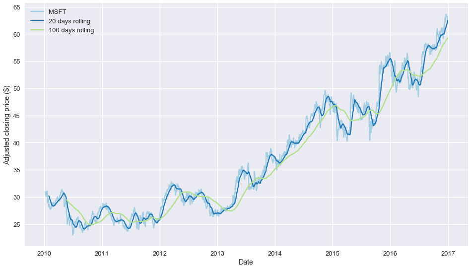
Now, we finally the stock price history together with the two moving averages plotted!
What's Next
All of this has been but a small preview of the way a quantitative analyst can leverage the power of Python and pandas to analyze scores of financial data. In part 2 of this series on Python and financial quantitative analysis, we are going to show how to use the two technical indicators already created to create a simple yet realistic trading strategy.
Continue Learning
- Python for Financial Analysis and Algorithmic Trading (Udemy)
Goes over numpy, pandas, matplotlib, Quantopian, ARIMA models, statsmodels, and important metrics, like the Sharpe ratio
Meet the Authors

PhD in Applied Mathematics and Statistics. Analyst working on quantitative trading, market and credit risk management and behavioral modelling at Barclays Investment Bank. Founder and CEO of QuAnalytics Limited.